Introduction
I’m a big fan of building Box and Whisker plots (also known as Box plots to those in the statistics world) to interpret certain data sets. While I tend to use these for charting Power Query refresh times, they really can be used for anything where you are trying to understand the variation of your results. The only criteria is that the values should be numeric like daily sales, number of warranty returns, air quality indices, or temperatures for example. These charts offer a lot of information – if you know how to interpret them. (And if you don’t… have a read of this article which explains exactly how these charts work!)
Preparing your data for a Single-Series Box and Whisker plot in Excel
In order to create a Box & Whisker chart in Excel, the first thing we need to do is make sure that our data is in the proper format. Fortunately, this is pretty easy, as we just need a single column of numbers that represent our numeric observations.
NOTE: These charts really need a minimum of 4 observations in order to render all the elements properly. Having said this, they are really intended to be used with many more data points in an effort to draw reasonable conclusions. I’m not going to go in to methods of how to determine your ideal sample size to make your data statistically significant as that is a whole other discussion.
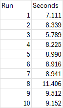
For this post, I’m going to use a short data set of 10 observations that represent some Power Query refresh times, as shown here:
Building a Single-Series Box and Whisker plot in Excel
Creating the chart is fairly straight forward. Here’s what I did:
- Selected the data and pressed CTRL + T to turn it into an official Excel table. (To be fair, this is an optional step, but makes it easier to update the chart in future when you add more data, as new rows pasted into the table will automatically be included in the chart.)
- Selected the entire “Seconds” column I was interested in plotting
- Went to Insert -> Recommended Chart -> All Charts -> Box & Whisker -> OK
NOTE: With Monkey Tools installed, I was also given the ability to rename my table immediately. I called my table “Data”. If you don’t have Monkey Tools installed (which you should as this is a free feature), you can still do this by selecting your table and going to the Table Design tab. On the far left you’ll find your table name which you can change.
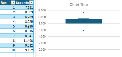
The result is a Box & Whisker chart that… needs some work…
I then customized the chart immediately as follows:
- Change the Chart title to something meaningful. (This is important to give your data context and remind you of the story you are trying to illustrate.)
- Right click the box and change the Fill colour to something lighter so that you can actually see the items on the chart.
After making these changes, I now have a readable box plot that looks like this:
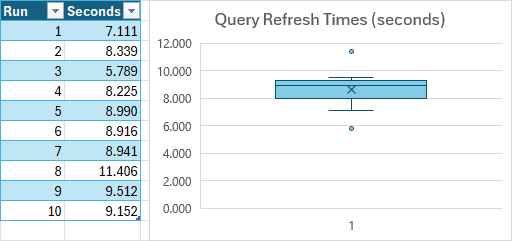
Believe it or not, that's all it takes to create a Box & Whisker plot... it is now ready to be interpreted. (And don’t forget that we have an article to help with exactly that!)
Building a Multi-Series Box and Whisker plot in Excel
Building a multi-series Box & Whisker chart is quite similar to building a single series version – as long as your data is in the correct format. In the image below, you can see how we need to keep things organized:
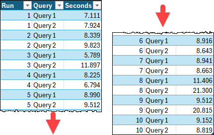
What you’ll notice in the above is:
- I have kept my data formatted as a table. (Again, this is optional, but highly recommended as it makes it super easy to add new data points due to the Table’s automatic expansion ability. Simply paste your new observations in the row immediately below the existing data, and it will automatically expand and pull it into the chart.)
- I have added a column to hold the series name that each of the data points is applicable to.
Now, let’s create the multi-series Box & Whisker chart:
- Select the data in the Series and Value columns (Query and Seconds in this case)
- Go to Insert -> Recommended Chart -> All Charts -> Box & Whisker -> OK
- Change the Chart title to something meaningful
- Right click the blue fill and change it to any lighter colour (of your choice)
Here’s the results that I generated:
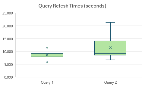
As you can see, each series is displayed separately, allowing you the ability to make comparisons between them.
Box & Whisker Configuration Options
To be honest, I usually only soften the fill colour of the charts to make them more readable and leave the rest of the chart configurations at their default states. Having said that, there are a few options available for these charts that you may wish to try. To configure them, right click one of the boxes and choose Format Data Series. In here, you will find a few options worth calling out:
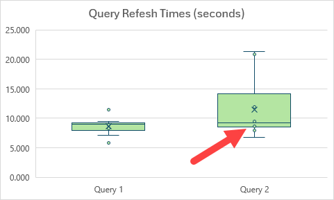
Option: Show Inner Points
Personally, I can’t say I’m a fan of this option as I find it adds clutter, makes the chart too noisy, and invites too many questions as to why these points vs others. Regardless, here is what it looks like on our sample chart:
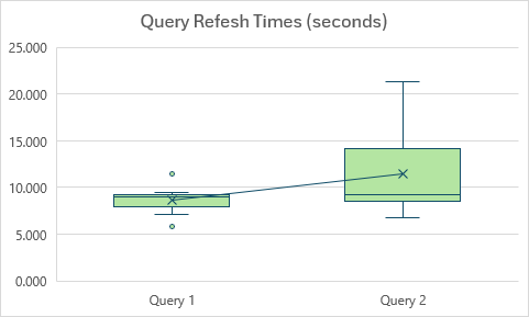
Option: Show Mean Line
The Show Mean Line option allows you to add a line connecting the mean points between series. Personally, I wouldn’t do this often as I feel that - if you are truly interested in a difference of means calculation - you probably want the exact values. But if your goal is to give a quick visual idea of variation between mean values, this will provide an indicator as to the relationship between the two.
Inclusive Quartile Calculation
By default, Excel’s Box and Whisker charts are drawn using an Exclusive Quartile calculation. Ignoring the exact mathematics of the calculations, the effective difference between using Inclusive and Exclusive quartiles is that Inclusive result in a narrower interquartile range with more outliers as shown here.
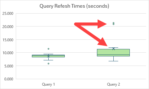
Notice how – compared to our previous chart – the maximum for Query 2 has moved from ~21 to ~12, and the values around 20 seconds are now shown as outliers.
Conclusion
As long as your data is in the correct format, building Box & Whisker charts in Excel is actually pretty straight forward. And now that you’ve built your Box & Whisker chart…
- Do you know how to interpret Excel’s Box and Whisker chart?
- Do you want to prove out the values used in Excel’s Box and Whisker chart?