I had an email exchange with Charley Kyd tonight, and I was bemoaning the fact that I couldn't link my Excel chart titles to a range. I could have sworn you could do this, but not working with charts a ton, I just could not find a way to do this in the Excel 2010 user interface.
To me, the logical place for this kind of functionality would be in the "Select Data Source" userform. This would seem a no-brainer since it's where you link up your series, define your chart range and axis labels as well as your legend. Why wouldn't you be able to link your title here if it was possible?

Well, apparently, just because it isn't in a wizard or a userform doesn't mean it can't be done... and done without resorting to VBA.
What I was looking for specifically was to give the following chart a dynamic title.
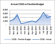
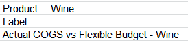
The data in the table is dynamic, and reflect the product line. So depending on a data validation list, I could be showing Beer, Wine or Liquor sales. Based on what Charley told me, I set up a little matrix under the chart:
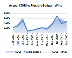
Next, I:
- Select the chart title
- Press =
- Click on the cell that contains my new dynamic title
And voila!
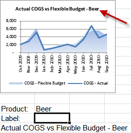
And likewise when I change it to reflect Beer:
So am I the only person who didn't know this? It's not really that intuitive is it? (Thanks for the pointer, Charley!)
5 thoughts on “Linking Excel Chart Title to a Cell”
I think Rob Bovey's XY chart labeller essentially does the same thing with Data Labels.
"So am I the only person who didn’t know this?"
I'm afraid so. 😉
At least, the only one who was brave enough to admit it, anyway. 😉
Not sure how far back this goes, but I remember it was already available in Excel 5 (talking 1995 here) 🙂
Same goes for axis titles too.
I must admit I tend to hit F2 then type the formula, including cell refs or whatever, not sure I've ever done it just by starting to type the equals sign, so you have saved me a key press there!