In this post I’m going to show one of my favourite financial modeling tricks: how to use Aggregate to Count Visible Rows.

Background

Often, when I’m building models in Excel, I like to group key assumptions at the top of the worksheet in one area. This allows me to change them easily from a centralized location. The problem is that sometimes I need to collapse them to see more of the model.  Of course, you can use this trick to collapse any block of rows (or columns) in your worksheet, so it’s applicable to all kinds of uses.

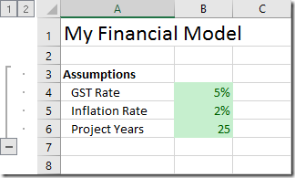
Let’s take a look at the basic setup:

So it’s essentially a block of cells to capture key rates and stats.  No secret there.  And on the left I’ve added some outlining so that I can collapse it easily.  To do that we simply select rows 3:6 and go to Data –> Outline –> Group.

The Trick in Action

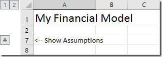
Now, check this out… I click the – on the left, and the rows collapse.

But check out the message in cell A7.  It wasn’t there before, but now we’ve got a nice message that not only tells you there is an area that is collapsed, it also leads the user as to how to show the rows again.

Using Aggregate to Count Visible Rows

The trick to this is using the AGGREGATE function (which works in Excel 2013 or higher).  So let’s check out how this works.

As AGGREGATE gives us back a count of rows, we will be able to test if the number of visible rows equals zero, and the react to it using an IF function.  So let’s get started.

AGGREGATE's first parameter: the Aggregation Type

=IF(AGGREGATE(

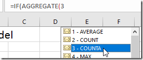
When we open the parenthesis, we are prompted for the first parameter.  There are a variety of options here, but the one I want is COUNTA(), which allows us to count the number of completed cells (either text or values):

Next up we put in the comma and we’re on to the second parameter.

AGGREGATE's second parameter: What to aggregate

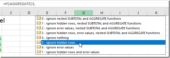
Aha!  So using 5 will allow us to apply the COUNTA(), but ignore any hidden rows.  So it’s this parameter here that allows us to use AGGREGATE to count visible rows only.

AGGREGATE's third parameter: The data to aggregate

On to the next comma and now we need to select the range to count.  Now in this part we have two options.  Personally, I prefer to provide the range of the cells that will be hidden.  In truth though, you only really need to refer to a single cell in the range that will be collapsed.  Here’s what I went with:

=IF(AGGREGATE(3,5,A3:A6

Wrapping up the IF test

Perfect, and now we can just close the parenthesis and complete the test:

=IF(AGGREGATE(3,5,A3:A6)=0,

So, if the count of visible cells equals zero then… what do we want to do?

The IF test: If there are no visible rows...

This is the part that I think really makes this trick work.  I really like providing the arrow key to point to the + icon that shows up, and adding the additional wording as needed.  This allows my users to know not only that there is hidden data, but how to display it again.  So for me, that message might look like:

• “<-- Show assumptions”
• “<--Click to expand Revenue assumptions”

You get the idea.  For this example I’ve gone with the following:

=IF(AGGREGATE(3,5,A3:A6)=0,“<-- Show assumptions”,

The IF test: If there are visible rows...

And finally, we round it off with the messaging to provide if the count of visible rows is greater than zero (i.e. if the section is expanded).  Depending on what you want your model to do and how you want to display things for your end users, this could be something like:

• “End of Assumptions”
• “Total Revenue”
• “Please insert new rows above this line”
• “”

I think the first three are fairly self explanatory, but the last one is essentially two sets of double quotes.  Since everything between the quotes is returned to the cell as text, and there is nothing between the quotes, we get an blank cell.

The complete formula to use Aggregate to Count Visible Rows

Using that method, the finalized formula reads as follows:

=IF(AGGREGATE(3,5,A3:A6)=0,“<-- Show assumptions”,””)

Final Thoughts

My clients love this little trick. It’s fairly easy to set up, and is super useful for allowing people to hide/show the model sections that they want/need to review, without having them bogged down with all the info.

I also find it very useful when we’ve got multiple scenarios laid out on the worksheet. Say I need to look at… scenario 1 and 3 at the same time, I can compress 2 and just focus on the stuff I need to look at, avoiding scrolling up and down.