What are Styles?
A style is pre-defined set of formatting instructions held together in one convenient package. They can be configured to apply one, two or many formatting characteristics, and can be applied to a worksheet cell or range very easily.
Why Use Styles?
The biggest reason that you'd want to use styles is their ease of use when you want to update a cell, be it a color/colour change, number style or font. If you have a style set up, you simply need to change it in one place, and every other cell in your entire workbook that uses that style is updated with it. We'll work through an example to show how these benefits can be used to our advantage.
Some useful things that can be done with styles might include:
- Unlocking and shading all data entry cells
- Providing consistent formats for controlling text vs date vs numerical input masks
- Locking all business logic (formula) cells
The key is that once your cells are tagged with a specific style, you never have to worry if you've updated all of them when you make a change. By virtue of using the style, you have enforced some consistency across your workbook. (Never again worry about that one key formula that you forgot to protect!)
Another benefit is that by designing styles, you force yourself to think a bit more about your workbook design. This may be a bit frustrating at first, but once you come to know what your basic data styles are, it actually becomes easier in the long run. Regardless, the benefits that you can reap from Style design far outweigh the cost and discomfort with getting used to them.
Finally, it can help with avoiding the dreaded Too Many Formats error message. Styles help organize and consolidate your formatting, eliminating much of the hodge-podge formatting that many of us do. Each of those formats is counted as a different item, and when you get too many the error message rears it's ugly head. I've been involved in a job that cost someone several hundred dollars to fix their workbook for this issue. Save yourself the time and money; use Styles.
Do Styles have Drawbacks?
Sure. You have to think about your workbook. Personally, I believe that proper planning is essential to good spreadsheet design, but many users are not used to it. Over time, though, it gets easier. We're going to save you some thinking to start with, so read on and save yourself some of that learning curve.
The other drawback that you'll feel is the time to set them up. It's so much easier to just jump in and start formatting what you want. Again, good planning yields superior results in the long run.
Using Styles
All right, so enough with the why and let's get on to the how.
Creating Styles
To create your own style in Excel 2003, go to Format-->Style. In Excel 2007, go to the Home tab and click the arrow in the bottom right corner of the Styles group as shown below:

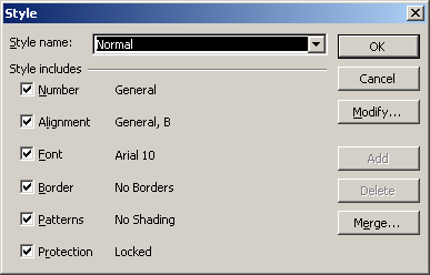
At this point it will pop up the Style dialog. (The Excel 2003 version is shown below.)

To begin with, give your new style a name. For this purpose, let's create a style that we'll use for all numeric data entry fields. Call it DE_Numbers.
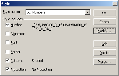
Each of the check boxes signifies which properties the style will control. Since this is a data entry cell, we want to control the number format, the pattern (we'll shade data entry cells) and also we'll want to make sure the cells are not protected. We're not really interested in overruling the font, alignment or borders, so un-check those boxes.
Now, click the Modify button (Excel 97-2003) or the Format button (Excel 2007) so that we can set the exact properties we want for each of these areas. You'll be taken to the "Format Cells" dialog.
- First, we'll set our number format. Choose the Accounting format, and change the $ sign to "none".
- Next, activate the Patterns tab. I tend to use a light green for data entry cells, as I find that it is easy on the eyes, and makes it easy for users to identify where data entry cells are. (I tell all my users that Green means Go.)
- Finally, we need to make sure that the cells are unlocked. Click the Protection tab, and uncheck the "Locked" box. (Of course, this setting won't take noticeable effect until the worksheet is protected.)
- Click OK to be returned to the Style dialog
Your dialog selection should now look similar to the following:

As you can see, we have chosen a specific number format, selected a shaded pattern, and decided to force all cells with this style to be unprotected, thereby allowing the user to enter data.
The final steps in creating the style are to click the Add button then Close to be returned to the worksheet.
You should now see that the worksheet cell you have selected is shaded in a light green. The style has been applied! You can prove this out as well by entering a number. It should automatically format to the number format you chose when setting up the style. Right clicking on the cell and going into the Format Cells dialog will show each of the options you chose as being selected.
Applying Styles
Applying styles in Excel 2007 is very easy. You simply select the cell (or range of cells,) then click your style in the Styles gallery on the Home tab.
Excel 97-2003 is a slightly different story. The native way to apply styles is to select the cell (or range of cells,) go to Format-->Style, pick the style from the list, and click OK. This is quite a few steps, which fortunately we can shorten.
To get a style picker on your 97-2003 toolbar, simply right click one of your toolbars and choose Customize (at the very bottom of the menu that will pop up.) Click the Commands tab, then select the Format category. From the right hand pane, locate the Style dropdown, left click it and drag it to one of your toolbars. As you can see, I've placed it on the Format toolbar.

At this point, you can quickly pick your desired style from the drop down list.
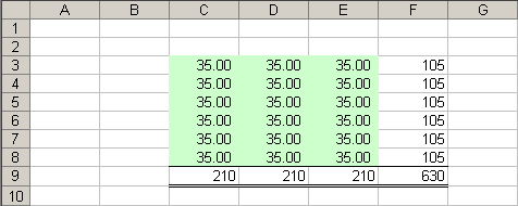
One thing that is worth mentioning here is how the style we created above actually applies across a range of data. In the image below, I formatted row 9 with a top border and double bottom border. I then applied our new style across cells C4:E8. Notice how the underline on row 8 does not disappear... If we had checked the borders box when creating our style, it would have forced our choice on these cells. Because we didn't, the existing borders have not been modified.

Updating Styles
Now this is where styles really shine... in the updates.
In Excel 97-2003, you select a cell with your style applied, go to Format --> Styles, and pick your style from the list. Excel 2007 is even easier, in that you just right click the Styles in the Home Tab's Styles gallery, and choose Modify.
At this point you can add/remove any categories and/or modify the individual settings. Let's make our numbers Bold and change the background to yellow.
- Check the Font box
- Click the Modify button (Excel 97-2003) or the Format button (Excel 2007)
- Go to the Font tab and select Bold from the Font Style selections
- Go to the Patterns tab and choose a yellow background
- Click OK to exit the Format Cells dialog
- Click OK again to exit the Style dialog
Voila! Every cell in your workbook that uses this style has now been updated, as shown below:
Strategic Moves
Why not set up your favourite styles, and make that workbook into a template? From there it's just a quick File-->New, (Office Menu --> New --> My Templates... in 2007,) and you have a workbook preloaded that you can use to build and deploy your projects!
See my Standard Styles
You can download an xlsx file that contains my most frequently used styles by clicking the button below. Each of the styles can be modified so that you can see exactly how they are all set up.


One thought on “Using Styles in Excel – Why and How”
Pingback: Excel Inter-Version Styles Quirk - Excelguru