Power Query is all about transforming and filtering data, and automating the process.  One of the tedious tasks that accountants get to deal with all the time is bank reconciliations, which is essentially the process of filtering and matching items to see what is left over.  It’s been on my list for a while now, but I’ve been thinking that we can use Power Query for listing outstanding cheques (or checks if you’re in the USA).

The completed workbook is available for download by clicking here.

Background

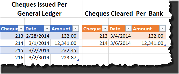
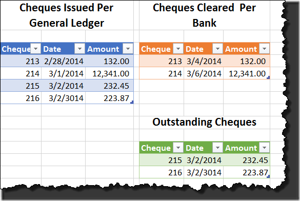
Because I don’t want to run on to 100 pages, I’m going to start with two lists that show just the cheques, in two tables:

The table on the left is the table of cheques that have been issued, as per the list maintained in the General Ledger. We’re making the assumption that we’ve dumped that list into an Excel worksheet, formatted it as a table, and given the table the name “GLListing”.

The table on the right is the table of the cheques that have cleared the bank.  Again, the assumption is that we’ve been able to download a list of the transactions, and filtered them down to show just the cheques that have cleared.  (Maybe we’d even use Power Query to do this.)  This table has been named “Bank”

Creating the data Staging queries

The first step is to create the staging queries to connect to these two tables.  One of the important things I wanted to ensure is that I can match transactions where both the cheque number and amount are identical.  (If a cheque clears for the wrong amount, I want to list it as outstanding at this point, as I need to review it.)  I’m going to keep that in mind as I create my staging tables.

The GLListing table:

To set this up I:

• Clicked inside the GLListing table –> Power Query –> From Table
• Set the data types on each column (Whole Number, Date, Decimal)
• Selected the Cheque and Amount columns –> Add Column –> Merge
  • Separator:  Custom (I used a dash)
  • Name:  Issued

The end result in Power Query:

• Go to Home –> Close & Load –> Close & Load To… –> Only Create Connection

The Bank table:

It’s virtually the identical process:

• Click inside the Bank table –> Power Query –> From Table
• Set the data types on each column (Whole Number, Date, Decimal)
• Selected the Cheque and Amount columns –> Add Column –> Merge
  • Separator:  Custom (I used a dash)
  • Name:  Cleared

The end result in Power Query:

• Go to Home –> Close & Load –> Close & Load To… –> Only Create Connection

Listing Outstanding Cheques

Now to build the important part.

• In the Workbook Queries pane, right click the GLListing query—> Reference

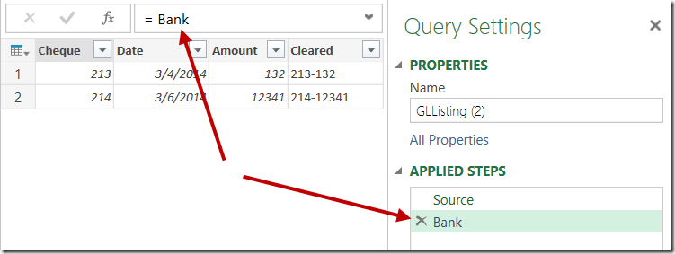
At this point you’ll have a pointer to the GLListing table.  We also want a pointer to the Bank table.  To do that, let’s click the fx icon on the formula bar:

This will create a new step in your query.  The formula in the formula bar will read =Source (it refers to the previous step), and you’ll see a new step in your Applied Steps area called Custom1.  Let’s update both of those:

• Change the formula to =Bank
• Right click and rename the step to “Bank”

The key things we now have are a Source step (which contains the output of the GLListing query) and a Bank step (which contains the output of the Bank query).  The Source step has an Issued column, the Bank query a Cleared column, and we’ll like to know which items between those two columns are different.

To work this out we’re going to knock up a little M code.  Here’s how:

• Click the fx icon on the formula bar
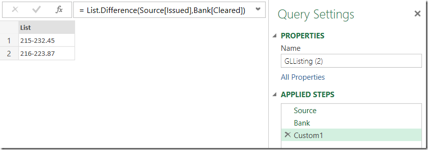
• Replace the formula (it will read =Bank) with this:

=List.Difference(Source[Issued],Bank[Cleared])

The result will be as follows:

So what happened here?  Let’s break this down.

List.Difference generates the items that are different between two provided lists.  And fortunately, when we feed a column to the function, it passes it in as a list.  So that’s what you’re seeing there:

• Source[Issued] is the Issued column from the Source step of our query
• Bank[Cleared] is the Cleared column from the Bank step of our query

And the result is the only items that don’t exist in both lists.

Expanding the Details

As great as this is, it is returning a list of values.  We want to convert this back into a table, and get the original data of issue as well.  So let’s do that.

• Go to Transform –> To Table

• When prompted, select that the list has a Custom Delimiter of a dash and click OK

You should now have a nice table split into two columns:

Let’s clean this up:

• Right click Column1 –> Rename –> Cheque
• Right click Column2 –> Rename –> Amount

Now, the next tricky part is getting the issue date back in.  I’d like to feed this from the current query – just to keep it self contained – but it’s easier to start by merging it with another query.

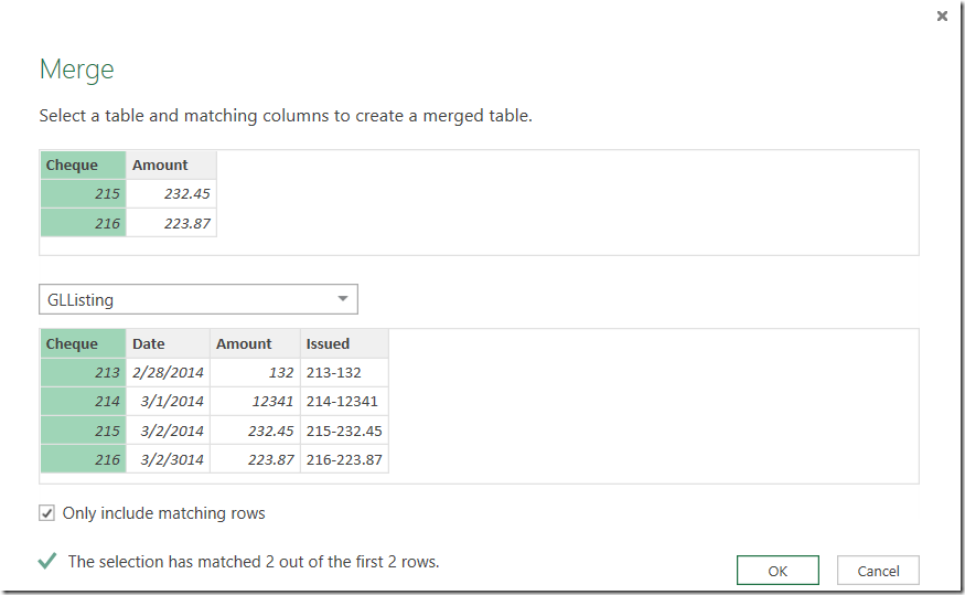
• Go to Home –> Merge Queries –> GLListing
• Choose to merge based on the Cheque field on both tables
• Make sure you check to “Only include matching rows”

• Click OK

This works nicely to add our column, but we’ve already pulled this data into this query once, so why reach outside it again?  If you look in the formula bar, you can see that the formula reads as follows:

= Table.NestedJoin(#"Renamed Columns",{"Cheque"},GLListing,{"Cheque"},"NewColumn",JoinKind.Inner)

Highlighted in the middle of the text is the name of the table we merged into this one.  So why not just replace that with the step name from this query that has the same table?  Modify the formula in the formula bar to read:

= Table.NestedJoin(#"Renamed Columns",{"Cheque"},Source,{"Cheque"},"NewColumn",JoinKind.Inner)

It doesn’t look like anything happened, does it?  That’s okay.  Remember that the source step just pulls in the data from the GLListing query.  Since we didn’t do anything to it in that step, it SHOULD look identical.

Now we can continue on and finalize the query:

• Expand the “NewColumn” column:
  • Only expand the Date column, as we have the others we need
  • Uncheck the “Use original column name as prefix” setting
• Move the Date column between then Cheque and Amount columns

• Rename the query to “Outstanding”
• Go to Home –> Close & Load

And the final result:

Final Thoughts

Figuring out which records match is actually pretty easy.  We simply merge two tables, and choose to only include matching rows.  Working out differences is obviously a bit harder.  (Wouldn’t it be awesome if there was an inverse setting on that merge dialog that let us only include unmatched rows?)

I left my full time controllership job before I ever got the chance to implement this technique for our bank reconciliations.  Currently there is a lot of VBA and manual work needed to clear both the cheques and deposits on a monthly basis.  Given this, however, I know that I could have re-written the bank reconciliation to very quickly eliminate all the records that match, leaving me with only the transactions that I actually needed to focus on.

Taking it even one step further, with another table of adjustments added in to the mix, I’m sure I could build it to actually produce an ever diminishing listing of un-reconciled transactions, and most likely even an output report replicating a full bank reconciliation.  Pretty cool, especially when you consider how much could be refreshed when you start the process next month!