I’ve posted on consolidating worksheets before, but in a task I got asked to do last week, I took a slightly different approach.  This approach allows consolidating worksheet print areas to grab the data that I need.

Background

In the previous post, I used some custom M code to reach outside the current workbook, and attach to the cached copy of the same workbook to read the data.  It works, but it’s a bit ridiculous that you need to.  One of the problems with that approach is that new sheets don’t show up in your solution until you save the workbook and refresh the query.  Not a big issue if you safeguard against it, but it’s a gotcha you want to be aware of.

In the situation I was working through, I wanted to consolidate some of the worksheets in the workbook, and also wanted to “future proof” it for new sheets that would be created later.  But I also wanted to make sure that all sheets would be pulled into the solution, even if they’d been newly created and the workbook hadn’t been saved.

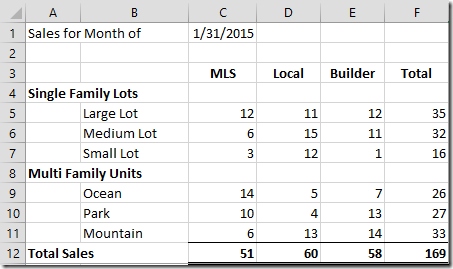
So my data (which you can download here) looks like this:

Yes, that’s right.  It’s pivoted, even though it’s not in a Pivot Table.  And I’ve got one sheet per month.  Naturally we’d like to turn this into a proper data source.

My Approach

I decided to go seriously hardcore, and just went right into a blank query:

• Power Query –> From Other Sources –> Blank Query

Not much to see yet (it is a blank query, after all) but I typed the following into the formula bar (which you can activate from the “View” tab if it’s not there.)

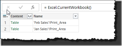
• =Excel.CurrentWorkbook()
• Enter

And check that out… I set some print areas!

What is in Excel.CurrentWorkbook()?

The Excel.CurrentWorkbook() command (and yes it is case sensitive) will give you a list of all tables, named ranges and power queries that are stored in your workbook.  And, as it happens, I can take advantage of this.  Because the print range is a named range, I can employ that to pick up my data.

Now, to be fair, I TOTALLY wish that Excel.CurrentWorkbook() also included all the raw worksheets.  That would be awesome.  You can get them by going to Excel.Workbook(File.Contents(full_file_path)) but that means it grabs them from the last saved version of the file in the workbook path.  Not ideal if your data is “live”.

At any rate, I’m good now.  So long as my users copy the previously set up sheet each month, and rename it to the current month, it will inherit the print area.  I now have something I can work with.

Consolidating Worksheet Print Areas

So let’s make use of this…

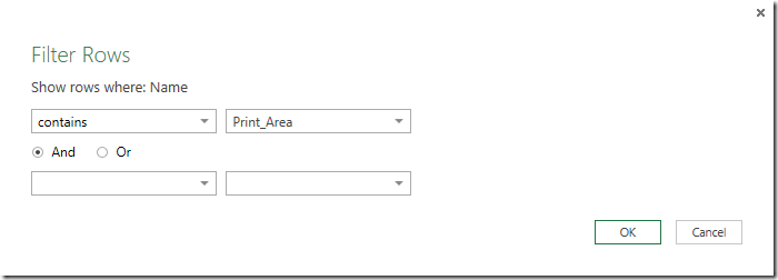
Something we need to recognize is that – as soon as we load this query to the worksheet – we are going to get a query and a table showing up in this list.  So let’s protect against that.  Click the Filter area on the “Name” column, and filter to records that contain “Print_Area”.

Now I don’t actually need the worksheet name for anything here, so I can

• Select the Name column –> Right Click –> Remove
• Click the Expand button (at the top of the the Content column)
• Un-check the option to use original column name as prefix and click OK

And I’m left with this:

So now it’s just time for cleanup.  Let’s do that:

• Go to Add Column –> Add Custom Column
• Call the column Date and enter the following formula:
  • if Text.Start([Column1],5) = "Sales" then [Column3] else null
• Select the Date column –> Transform –> Fill Down
• Go to Home –> Remove Rows –> Remove Top Rows –> 2
• Go to Transform –> Use First Row as Headers
• Rename:
  • “Column1” to “Major Group”
  • “Column2” to “SubClass”
  • “Column7” to “Date”
• Select the “Date” column –> Transform –> Data Type –> Date
• Select “Major Group” column
  • Go to Transform –> Fill Down
  • Filter to only rows that “does not contain” “Sales”
• Select “SubClass”
  • Filter to remove “null” records
• Remove the “Total” column
• Select the “Major Group”, “SubClass” and “Date” columns
• Go to Transform –> Unpivot Columns –> Unpivot Other Columns
• Rename
  • “Attribute” to “Category”
  • “Value” to “Units Sold”
• Rename the query to “Sales” and load it to the worksheet

Create a Simple Pivot

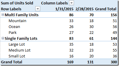
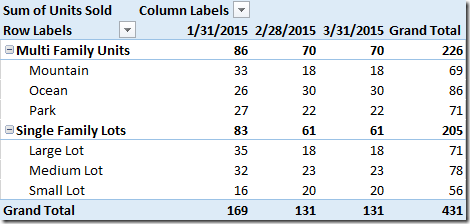
Now that we have our data, we can create a simple Pivot Table from it:

Which is great, but what about next month?  Let’s see what happens…

• Right click the “Feb Sales” worksheet –> Move or Copy
• Check the “Create a copy” checkbox and click OK
• Change C1 to 3/31/2015

Yuck… we’re simulating that we can’t trust our users to even rename the worksheet properly, but the do get the data right.  Now let’s see how our query reacts…

Go back to the Power Query worksheet, refresh the query, and the Pivot Table if necessary…

Awesome!

What’s Safe?

This worked because we only have the print area defined for our input sheets.  If someone added a print area on other worksheets we’d have to add additional/adjust our logic to deal with that, as we’d get data in our query that possibly shouldn’t be there.

If someone adds something outside the print area, then you have an issue.  In those cases a table may be a better option to start with.  And naturally tables also show up in the Excel.CurrentWorkbook() call.  Having said that, it’s harder to control the default names there, so that could be an issue for you.

If someone modifies the shape of a range, that could also be a problem.  Say a new column gets added or something.

At the end of the day you need to think through an anticipate the scope of what your users are likely to do, and what shape the data will likely stay in (or not) so that you can plan accordingly.  In the scope of the solution that I built, I’m fairly certain it will work without a challenge.