Creating a VLOOKUP Function in Power Query

2015-01-28
Ken Puls
Categories: Excel, Power BI, Power Query

Tonight I decided to actually follow through on something I’d been musing about for a while: building a full fledged VLOOKUP function in Power Query. Why? Yeah… that’s probably a good question!

Replicating VLOOKUP’s exact match is REALLY easy in Power Query. You simply take two tables and merge them together. But the approximate match is a little harder to do, since you don’t have matching records on each side to merge together.

Now, to be fair, you could go the route of building a kind of case statement, as Chris Webb has done here. In actual fact, you probably should do that if you want something that is lean and mean, and the logic won’t change. But what if you wanted to maintain a table in Excel that holds your lookup values, making it easy to update? Shouldn’t we be able to take that and use it just like a VLOOKUP with an approximate match? I don’t see why not. So here’s my take on it.

Practical Use Cases

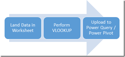
I see this as having some helpful use cases. They’ll mostly come from Excel users who are experienced with VLOOKUP and maintain lookup tables, and reach back to that familiarity. And they would probably be tempted to do something like this:

The concern, of course, is that landing data in the worksheet during this cycle contributes to file size, memory usage and ultimately re-calc speed, so if you can avoid this step on the way to getting it into Power Pivot, you plainly want to do that.

The cool thing is that by building this the way I’ve done it, you’re not restricted to landing your data in the worksheet to use VLOOKUP with it. You can pull data into Power Query from any source (csv, text file, database, web page) and perform your VLOOKUP against your Excel table without that worksheet round trip.

Let’s Take a Look…

Now, I AM going to use Excel based data for this, only because I have a specific scenario to demonstrate. You can download a sample file – containing just the data – from this link. (The completed file is also available at the end of the post.)

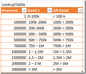
So, we have a series of numbers, and want to look them up in this table:

I really used my imagination for this one and called it “LookupTable”. Remember that, as we need that name later. Note also that the first record is 1, not 0. This was done to demonstrate that an approximate match can return a #N/A value, as you’ll see in a minute.

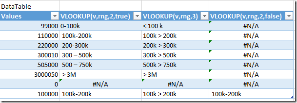
Now here’s what things would look like using standard Excel VLOOKUP formulas against that table:

Hopefully this makes sense. The formulas in columns 2, 3 and 4 are:

=VLOOKUP([@Values],LookupTable,2,TRUE)
=VLOOKUP([@Values],LookupTable,3)
=VLOOKUP([@Values],LookupTable,2,FALSE)

Just to recap the high points here… column 2 declares the final parameter as ,TRUE which will give us an approximate match. Column 3 doesn’t declare the final parameter, which will default to ,TRUE and give an an approximate match. Column 4 declares the final parameter as ,FALSE which means we’ll want an exact match. The end result is that only one value matches, which is why we get all those #N/A results.

Standard VLOOKUP stuff so far, right?

Creating the VLOOKUP function in Power Query

Before we get to using the function, we need to create it. To do that we’re going to go to:

Power Query –> From Other Sources –> Blank Query
View –> Advanced Editor

Highlight all the code in that window and replace it with this… (yes, it’s not short)

let pqVLOOKUP = (lookup_value as any, table_array as table, col_index_number as number, optional approximate_match as logical ) as any =>

let 
/*Provide optional match if user didn't */
matchtype =
if approximate_match = null
then true
else approximate_match,

/*Get name of return column */
Cols = Table.ColumnNames(table_array),
ColTable = Table.FromList(Cols, Splitter.SplitByNothing(), null, null, ExtraValues.Error),
ColName_match = Record.Field(ColTable{0},"Column1"),
ColName_return = Record.Field(ColTable{col_index_number - 1},"Column1"),

/*Find closest match */
SortData = Table.Sort(table_array,{{ColName_match, Order.Descending}}),
RenameLookupCol = Table.RenameColumns(SortData,{{ColName_match, "Lookup"}}),
RemoveExcess = Table.SelectRows(RenameLookupCol, each [Lookup] <= lookup_value),
ClosestMatch=
if Table.IsEmpty(RemoveExcess)=true
then "#N/A"
else Record.Field(RemoveExcess{0},"Lookup"),

/*What should be returned in case of approximate match? */
ClosestReturn=
if Table.IsEmpty(RemoveExcess)=true
then "#N/A"
else Record.Field(RemoveExcess{0},ColName_return),

/*Modify result if we need an exact match */
Return =
if matchtype=true
then ClosestReturn
else
if lookup_value = ClosestMatch
then ClosestReturn
else "#N/A"
in Return
in pqVLOOKUP

Now:

You can alternately download the M code from my OneDrive.
Click Done
Change the Name (top right under Properties) to “pqVLOOKUP”
Click Home –> Close and Load

All right… the function is there. Now let’s go make use of it… (we’ll come back to how it works in a bit.)

Using the VLOOKUP function in Power Query

Now, before we go any further, I want to ask you a favour. I need you to pretend for a second. Pretend that the data we are connecting to next is a database, not an Excel table. You’ll see how this can be useful if you’ll play along here. (The only reason I’m using an Excel table for my source data is that it’s easier to share than a database.)

Let’s go click in the DataTable table. (This one:)

Now, let’s upload this “database” into Power Query…

Go to Power Query –> From Table

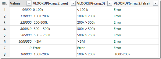
You should have something like this now:

Funny how Power Query reads the #N/A values as errors, but whatever. Let’s get rid of those columns so that we’re left with just the Values column.

Right click Values –> Remove Other Columns

Now, we’re going to make a really small M code edit.

Go to View –> Advanced Editor
Copy the second line (starts with Source =…)
Paste it immediately above the line you just copied
Modify it to read as follows:
- Source –> LookupSource
- DataTable –> LookupTable

Your M code should now look as follows:

Click Done

Nothing really appears to look different right now, but you’ll notice that you have an extra step called “LookupSource” on the right. If you switch back and forth between that and Source, you’ll see we are looking at the original DataTable and the LookupTable. The reason we do this is to make the next step really easy.

Go to Add Column –> Add Custom Column
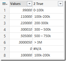
Call the column 2 True
Enter the following formula:
- pqVLOOKUP([Values],LookupSource,2,true)

Okay, so what’s what?

pqVLOOKUP is the name of our function we added above
[Values] is the value we want to look up
LookupSource is the table we want to look in to find our result
2 is the column we want to return
true is defining that we want an approximate match

And, as you can see when you click OK, it works!

Let’s do the next two columns:

Go to Add Column –> Add Custom Column
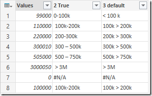
Call the column 3 default
Enter the following formula:
- pqVLOOKUP([Values],LookupSource,3)

So this time we asked for a return from the 3rd column, and we omitted the final parameter. Notice that it defaulted to true for us:

Last one…

Go to Add Column –> Add Custom Column
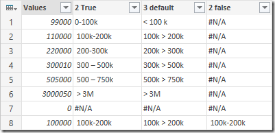
Call the column 2 false
Enter the following formula:
- pqVLOOKUP([Values],LookupSource,2,false)

And how about that, all but one comes back with #N/A:

And with that you can load this into a table in the worksheet:

Notice that the results are identical to that of the original Excel table, with one exception… the #N/A I have provided is text, not an equivalent to the =NA() function.

The completed file is available here.

How Does the VLOOKUP Function in Power Query Actually Work?

This VLOOKUP actually has some advantages over the VLOOKUP we all know and love. The most important is that we don’t need to worry if the list is sorted or not, as the function takes care of it for you. It essentially works like this:

Pull in the data table
Sort it descending by the first column
Remove all records greater than the value being searched for
Return the value in the requested column for the first remaining record UNLESS we asked for an Exact match
If we asked for an Exact match then it tests to see if the return is a match and returns #N/A if it’s not

Some key design principles I used here:

The parameters are all in EXACTLY the same order as Excel’s VLOOKUP
The required, optional and default parameters match what you already know and use in Excel
The function is dynamic in that it will work no matter what your lookup table column names are, how many rows or columns it has
It returns results that are in parallel with Excel’s output
The function is pretty much a drag’n’drop for your project. The only thing you need to remember is to define the lookup table in the first part of your query

So how cool is that? You love VLOOKUP, and you can now use it in Power Query to perform VLOOKUP’s from your Power Query sourced database queries against tables of Excel data without hitting the worksheet first! (In fact, if your database has an approximate table, you could VLOOKUP from database table against database table!)

60 thoughts on “Creating a VLOOKUP Function in Power Query”

Jon Acampora on January 29, 2015 at 12:18 pm said:

Hi Ken, This is a great post! I have a model where I'm going about this the old way of landing the data in the file, then doing the vlookup. This is a much more efficient approach.

I have a question about the error handling. You are returning the "#N/A" text within the function if it is an error. What is the best way to further evaluate the error? In Excel you could use IFERROR. In power query would you just use an IF Then statement, or is there a better way to handle errors?

Thanks again!
Ken Puls on January 29, 2015 at 1:54 pm said:

Hey Jon,

It depends on what kind of error handling you're looking for, really. You could test for the #N/A as follows:
= if [ColName] = "#N/A" then < do something > else < do something else >

We're also not stuck to returning #N/A, of course. We could return null, "not found", or even an error if we wanted to.
Pingback: Excel Roundup 20150202 « Contextures Blog
Anthony Newell on March 25, 2015 at 5:44 am said:

Great stuff Ken. Would you be able to do similar to replicate the Match/Index functionality in Excel
or alternatively and more simply, replicate the LookUpValue function in PowerPivot
I just want to pass a search value, result column and search column
I've had a go but my brain went into meltdown / shutdown mode very quickly!
Amy Jo Bowers on August 11, 2015 at 6:46 am said:

Hi Ken,

Thanks for the post! I was able to replicate this successfully for my Power Query, which gets data from and Excel Table and a SharePoint List. However, since I've added the "pqVLOOKUP" column, refreshing my data takes much longer (approx. 2-3 seconds per line item). With over 10,000 line items, this takes quite some time, and this is only with one pqVLOOKUP column; I was planning on adding 10+ more. Any ideas of how to make my data load quicker? Thanks again!
Ken Puls on August 11, 2015 at 7:36 am said:

I guess the first question is "do you need an approximate match". It's the searching through all possibilities that takes the time. The other alternative would be to create a table with all possibilities in it, then merge the two (simulating a PQ VLOOKUP Exact match). My guess is that could be faster.
Roberto from Italy on September 3, 2015 at 9:58 pm said:

Hi, very interesting post! Great work.
I'm looking for something like index & match working into pq.
I have a table with different person in rows, "year&month" in coloumns (201501,201503,201504...): in every different cell I have a different name representin a workplace (place1,place2...)
Now, in my pq I have different rows and a coloumn containing name of person, a coloumn with year&month and I'd like to add a coloumn containing the work place corresponding to that person for that yearmonth. I can't find the way. Could help me?
Thanks in advance.
Roberto, Italy
Ken Puls on September 4, 2015 at 9:05 am said:

Hi Roberto,

The issue, I think, is the MATCH function. Index we could make work fairly easily, but the MATCH kind of depends on whether you are trying to match column headers or rows. Each of those needs to be handled differently in Power Query...
Roberto from Italy on September 5, 2015 at 9:29 pm said:

Hi Ken, thanks for your answer.
I try to explain me better. Table 1 contains different col with progression of "YearMonth" (201501, 201502...), and Rows with different "Person": every cell of the Table 1 contains a name that is a different work place (Place1, Place1, Place 1, Place 3, Place 3...).
Table 2 contains dataset from PQ: for each record there is a coloumn containig a "Person" and another containing "YearMonth".
The goal is to create a new Col in Table 2 containing, for each record, the name (Place1, Place2...) of the cell in Table 1 that BOTH Match with the "Person" (Row) and the "YearMonth" (Col) of that record.
In Excel I use INDEX and MATCH function that I can't manage in PQ.
Another solution could be create the new Col in PowerPivot? Is there the function?
Sorry for ALL these questions, and thanks for your very appreciated answer!
Roberto, Italy
Elias on September 6, 2015 at 9:36 am said:

Hi Roberto,
You can unpivot Table1 in Power Query (Select person column ->Unpivot other columns), then merge the results with table2 by Person & YearMonth.

Regards
Elias
Roberto from Italy on September 6, 2015 at 3:39 pm said:

Hi Elias,
Thank you so much.
I think it's a great idea. I have been able to do everything but near the end of the process of loading last files of the directory I use, Excel frozen....
I tried many times...the same. I cancel the cache, no way.
But I think it's the right method.
Thanks, I'll try again.
Roberto, Italy
Roberto from Italy on September 7, 2015 at 3:47 pm said:

Hi Elias and Ken,
IT WORKS! Wow...great tip!
Yesterday didn't because there was a file corrupted.
Thank you so much for your work and your blog.
Roberto
Tim on September 23, 2015 at 1:44 am said:

Thank you very much - your step-by-step guide was very informative and has saved me an immense amount of time!
AlexJ on September 30, 2015 at 4:17 am said:

Works a treat. Thanks - saved me hours/compromises.
duncan on October 7, 2015 at 8:56 pm said:

Thanks for providing this comprehensive and useful resource. Much appreciated.
George on January 19, 2016 at 8:56 pm said:

Hello
I also have a problem with #N/A error when trying to unpivot.
My original excel table contains #N/A errors (due to wrong mapping - that's fine). However, when I load this table into Power Query, it transforms these #N/As into "Error". If I want to unpivot this table I end up with Errors in all the columns of the rows that originally had a cell with "Error". The result is a nonsense because data is lost...
How can I load data into Power Query and tell it to treat all the N/As in original excel as text? Or how to let it ignore the errors in the source table when I try to unpivot?
Thanks for help,
George
Ken Puls on January 19, 2016 at 9:49 pm said:

Hi George,

After pulling the data in, select the columns that show the errors. Go to the Transform tab and choose Replace Errors. Replace it with #N/A and it should then treat it as text for you.

Hope that helps!
George on January 21, 2016 at 12:58 pm said:

Hi Ken, yes, that's very helpful.
Thank you very much!
Emma on February 2, 2016 at 1:54 pm said:

Hi Ken, I have a question about the performance issue. I have to handle master data with Vlookup function. Can I know which would perform better/ faster between power query and PowerPivot? Power query can do vlookup. PowerPivot can do relationship to achieve it. Thank you in advance
Ken Puls on February 3, 2016 at 11:03 am said:

Hi Emma,

Well... they're kind of apples and oranges. Power Query will take longer to load up front, but can avoid the memory required to hold a separate table in Power Pivot that needs to be linked. It's Power Pivot's memory usage that drives its performance.

If your model is loading slowly when you click a slicer, move to Power Query to shift the time to the refresh. If it works fine with slicers as is, do the work with relationships in Power Pivot.
JDoe on February 29, 2016 at 7:11 am said:

Hi Ken,

I had a vlookup table of all possible options and what to classify them as, now power query correctly simplifies down all possible options into 12 groups, but I still get ten million records coming back as (blank) even though my pivot table says to classify (blank) as Group Misc, is there something else I need to do in order for power query to capture blanks and convert them in the query? Thank you.
Ken Puls on February 29, 2016 at 5:47 pm said:

Hey there,

So one thing I'd be curious on is if you are seeing a disconnect between blank and null. Those are not the same in Power Query and might be a place to start looking. The other thing to recognize is that Power Query is case sensitive, which could lead to mismatches as well unless you deal with that in your M code.
Chris on March 7, 2016 at 7:38 am said:

Ken, this is brilliant! You never cease to amaze me. (Also, I love your book M is for (Data) Monkey)!

I have an extension of this question, perhaps you'd look?

Essentially I am trying to do a lookup against two variables, most notably a date. So, I'm trying to lookup an employee from an ID value and a date... The lookup table typically has several entries for each ID value at random dates (random as that there isn't a set number of days between them). The date value has to at least greater than or equal to the lookup table date, but less than any other later dates that may occur.

For example, we're looking up ID 12345 for the date of 1/20/2016, but the lookup table contains a row for ID 12345 for both 1/18/2016, and 1/22/2016. It needs to round down to the nearest date past the date value, returning the employee for ID 12345 on 1/18/2016.
Chris on March 7, 2016 at 11:52 am said:

I forgot to include what I've worked out so far...
It's quite basic, as I'm still learning about the syntax and details of PQ.
I'm using a custom function, but so far have only been able to return single values. Is it possible to return a table/record that can be expanded in the invoking query (like a Table.NestedJoin)? I would also ideally like the column "[ID]" set as a variable, so it can be used on alternate columns but I can't figure out the syntax...I even tried utilizing the column number by using your ColTable example, added an Index Column & filtered, but still couldn't figure out how to use it to refer to a column from within the function.
________________________
Function:
let
IDTest = (table as table, id as text, date as date) =>
try Table.Max(Table.SelectRows(table, each [ID]=
id and [Effective Date] <= date),"Effective Date")[Employee] otherwise null
in
IDTest
________________________
Invoking Query:
let
Sauce = LookupTable,
Source = DataTable,
LookDown = Table.AddColumn(Source, "LookDown",
each IDTest(Sauce, [ID], [Date]))
in
LookDown
Ken Puls on March 9, 2016 at 4:47 pm said:

Hi Chris,

You can absolutely return a table from a function. Set your function up to generate the table you want, then modify the query to put the word's "as table" right before the => portion of the function declaration.

For dynamically passing columns, Chris Webb just posted a blog post on that subject here which may help: http://blog.crossjoin.co.uk/2016/03/07/dynamic-column-selection-in-custom-columns-in-power-bipower-querym/
Hossein on March 11, 2016 at 7:14 am said:

How about using "Table.Buffer" for the "RenameLookupCol" part? I think it can enhance the speed of the function.

RenameLookupCol = Table.Buffer(Table.RenameColumns(SortData,{{ColName_match, "Lookup"}}))
Ken Puls on March 13, 2016 at 10:34 pm said:

It may, but I think you'd probably rather buffer the table before you call the function, not once you call it.

LookupSource = Table.Buffer(Excel.CurrentWorkbook(){[Name=LookupTable]}[Content],

I have not tested this though.
Neal Whittinghill on March 29, 2016 at 9:45 am said:

Great Blog! Please forgive me if this is not the correct thread to be posting in. I'm trying to wrap my head around this whole "M" language but I'm not quite there yet. I use the following excel function to find the last instance of "Serial #", and then it returns a value from the same row in the "Opr. short text" column.

=IFERROR(LOOKUP(2,1/(MASTER_DATA[Serial '#]=[@[Serial '#]]),MASTER_DATA[Opr. short text]),"")

I understand somewhat that the "IFERROR" portion might not be necessary and that the "M" Language does not use all caps. I'm just having a difficult time with my specific example converting this to something I can use in Power Query.
Am I heading in the right direction or is there another simpler method to attain the same result? I really appreciate the input! *My apologies, newbie here*
Simon on May 4, 2016 at 12:06 am said:

Hi Ken

What would be the drawbacks of the following approach to emulating an approximate VLOOKUP in a simple case:
Merge the two tables, setting the Join Properties to include all the records from the 'Many' table.
Sort the resulting table by the join/lookup column in the Many table.
Use Fill Down on that column to replace the nulls with the lookup values.

I've just started reading M is for (Data) Monkey - very useful and practical.
Simon on May 4, 2016 at 5:41 am said:

Further to my last question about Fill Down and VLOOKUP, I've just worked out a pretty obvious drawback for myself: it would only work if all of the lookup table's rows were matched in the Many table. To avoid this, I guess that the Join Properties would need to be set to Full Outer, and a custom column created using 'if' to return the value from the lookup table if the Many table equivalent was null. This would become the sort column and, once the relevant columns had been filled down, the lookup table rows could be filtered out (filter out nulls in the Many table join column).
Ken Puls on May 4, 2016 at 3:07 pm said:

Interesting approach. I'd certainly want to test and make sure it worked fully before I jumped on it. 🙂
Ken Puls on May 4, 2016 at 3:09 pm said:

Hi Neal,

Can you post your question in our Power Query forum at http://www.excelguru.ca/forums ? That would probably be a better place to work through it. Thanks!
Simon on May 4, 2016 at 11:03 pm said:

Thanks Ken. Will do.
ZileXa on September 20, 2016 at 7:54 am said:

For me, at first it did not work. The matched result in the added column was just 1 of the values for all rows. This was caused by my own LookupTable: the value to lookup should of course be in the first column! But even after I changed this, the problem remained: the pqVLOOKUP was probably already cached.

To solve this:
By hitting Close&Load, you end up back in Excel, now refresh the pqVLOOKUP connection and edit the other one (the query containing your tables), close and load it and voila!

Note that this part did not work for me:
LookupSource = Excel.CurrentWorkbook(){[Name="LookupTable"]}[Content],
It gave an error: table not found in the worksheet" or something like that, even though my workbook only contained 1 sheet, that exact sheet with the name LookupTable. I had to use this instead:
LookupSource = Csv.Document(File.Contents("C:\PathToFile\LookupTable.csv"),[Delimiter=",", Columns=2, Encoding=1252, QuoteStyle=QuoteStyle.None]),

Not sure why. But with a seperate file it did work.
ZileXa on September 20, 2016 at 7:59 am said:

I was actually looking for a VLOOKUP that would lookup a text VALUE and check if the LookupTable CONTAINS that text. Example:
VALUE to lookup: excelgurus.forlife
match if a row in the LookupTable is: excelgurus
match if a row in the LookupTable is: forever.excelgurus.ca
not a match if a row in the LookupTable is: excelllentbestgurus

I guess I need a different pqVLOOKUP formula. What could that be?
Ken Puls on September 20, 2016 at 11:18 am said:

You probably don't even need a custom function if you're looking for a specific term. If you're looking against a table of potential matches then you may. At any rate, the backbone to what you need is the Text.Contains() function: https://msdn.microsoft.com/en-us/library/mt253324.aspx
Shirley on October 5, 2016 at 11:38 am said:

Excellent post! Got it to work but refreshing the data takes much too long! My data table contains 36000 rows, my lookup table has 6000 rows.
Shirley on October 5, 2016 at 11:53 am said:

apologies for the double post...

Can you wrap pqVLOOKUPi in a condition statement?

while my data table has 36000 records, I am only interested in a VLOOKUP on the records with null/blank column values.

Will this reduce the time it takes to refresh the data?
Ken Puls on October 5, 2016 at 1:07 pm said:

Actually, there are two things you can do.

#1) Instead of using the LookupSource line like I did in the "Using the VLOOKUP function" part, replace it with this:
LookupSource = Table.Buffer(Excel.CurrentWorkbook(){[Name="LookupTable"]}[Content],

That will load the table into memory, rather than re-loading it in each call.

#2) Yes, wrap the pqVLOOKUP in a condition like this:
=if [Column1]=null then pqVLOOKUP([Column2],LookupSource,3,false) else [Column1]
mario on January 9, 2017 at 3:53 am said:

Great work,
may I suggest you to modify your script as below in order to manage correctly when is passed a col_index_number equal to 1?
ColName_return = if col_index_number = 1
then "Lookup"
else Record.Field(ColTable{col_index_number - 1},"Column1"),
Ken Puls on January 9, 2017 at 8:16 am said:

Thanks Mario, I'll have to try that out. Are you saying that the match doesn't come back correctly with a col index of 1 currently?
William on January 16, 2017 at 8:55 am said:

Hi Ken,

Found this post after reading about the revenue banding example in chapter 22 of your book. I have a very similar problem, but the pqVLOOKUP approach simply takes too long to load - I have ~75k rows of data and about 100 bands (1 band for every 30 days, all the way up to 8 years).

I'm leaning towards the solution you mentioned in an earlier comment: create a table with all the values, customize the bands through Excel formulas and merge them in PQ.
I also think a bunch of nested "else ifs" could be faster, but that would take a long time to write and the code would end up being huge.

Do you have any suggestions for this specific banding problem? Maybe there's an easier way in Power Pivot instead?

Thanks!
Ken Puls on January 16, 2017 at 9:00 am said:

Hey William,

I hear you here. Quick suggestion to try before you abandon this approach though....

Try changing the first line as follows:
LookupSource = Table.Buffer(Excel.CurrentWorkbook(){[Name="LookupTable"]}[Content]),

And if it's still too slow, try wrapping the Source line in Table.Buffer as well. You may find that those steps speed this up drastically.

Let me know,

Ken
Pingback: Power Query VLOOKUP Function – SELECT code FROM greycells
ajay on March 31, 2017 at 2:57 am said:

Hi Ken,

I am unable to evaluate the two dates by add the custom column, may be the dates are in text format and I can't change it at source level as other downstream transformation are effecting. Can you help me out here.

=if date1>= date2 and date1<date3 then
"ok' else "not'

remember the dates are in text format.

thanks
AR
Ken Puls on March 31, 2017 at 8:10 am said:

Hi Ajay,

You could try converting the columns to dates as follows:
=if Date.From(date1)>= Date.From(date2) and Date.From(date1)
drew bambic on January 13, 2018 at 2:20 pm said:

Ken --
§ an inline function that performs a range lookup on the 'LookupTable' described above is provided below
§ the "Alt Band" gets split into "From" and "To" columns
§ best of all - takes 5 lines of code.
§ with additional variables - this can be extended to perform both multi criteria matching in addition to the range lookups - all with very little additional code.
/*
let
DataTable2 = Excel.CurrentWorkbook(){[Name="DataTable2"]}[Content],
LookupTable2 = Excel.CurrentWorkbook(){[Name="LookupTable2"]}[Content],
fnCustom = (Band) => Table.SelectRows(LookupTable2, each Band >= [From] and Band <= [To]),
AddCol = Table.AddColumn(DataTable, "Custom", each fnCustom([Values])),
ExpandCol = Table.ExpandTableColumn(AddCol, "Custom", {"Band"}, {"Band"})
in
ExpandCol

Thanks - DrewBbc
Ken Puls on January 15, 2018 at 9:39 am said:

Cool stuff Drew. What's the performance like? I'm wondering if the first two tables should be buffered to speed things up.
Catalin Bombea on January 16, 2018 at 3:07 am said:

Another way to replicate the VLOOKUP function or the INDEX-MATCH combination in Power Query is :
GroupValue = (x) => List.Skip(Table.ToRecords(Table.Sort(Groups2,{{"Days", Order.Descending}})), each [Days] >= x){0}[Group],
#"Added Custom1" = Table.AddColumn(#"Changed Type2", "Buckets", each GroupValue([Days Past Due]))
The Groups2 Table has 2 columns: Days and Group (Age Groups like "31-62 days", to be more precise)
List.Skip will eliminate the records that does not meet the condition, and because multiple records may be returned, we keep only the first, indicating the column name from whitch the value should be returned:
List.Skip(...){0}[Group]

This approach will replicate an INDEX-MATCH formula, with "Less Than" match type:
=INDEX({"1-31 days ";"32-61 days ";"62-92 days ";"93-122 days";"123-153 days";"154-183 days ";"184-214 days";"215-244 days ";"245-275 days";"276-305 days ";"> 365 days "},MATCH(A1,{0;32;62;93;123;154;184;215;245;276;306},1))
Performance not tested...
Ken Puls on January 16, 2018 at 9:20 am said:

Awesome, thanks Catalin!
Haresh on May 15, 2018 at 10:25 pm said:

Hi Ken,
I am using your VLOOKUP to match transaction date in data table & Return Reporting dates from Lookup Table.
I use approximate match to get the nearest date.
Problem I am facing is that it returns date earlier than the transaction date whereas I need the Report Date that is nearest after the transaction date.
Please suggest a solution
Ken Puls on May 16, 2018 at 4:19 am said:

Haresh, this function is very slow for approximate match scenarios. You should try this one instead: https://www.powerquery.training/portfolio/vlookup-true-in-power-query/

If you have any challenges implementing this, maybe try posting in our forums at http://excelguru.ca/forums I'm sure we can help you out there.
Shay on December 22, 2018 at 3:29 am said:

BEUTIFUL!!!
I wanted to get rid of this #NA so I replaced then with a null in the the M code.

Thank you!
Sadiq Khoja on January 24, 2019 at 5:43 pm said:

DrewBbc / Ken,

Can we pass table to inline function? Something like this:

let
Lookup = Table.Buffer(Excel.CurrentWorkbook(){[Name="Lookup"]}[Content]),
Source = Excel.CurrentWorkbook(){[Name="DataTable"]}[Content],
fnCustom = (LookupTable,Band) => Table.SelectRows(LookupTable, each Band >= [Start] and Band <= [End]),
AddCol = Table.AddColumn(Source, "Custom", each fnCustom(Lookup,[age])),
ExpandCol = Table.ExpandTableColumn(AddCol, "Custom", {"Group"}, {"Group"})
in
ExpandCol
Ken Puls on January 24, 2019 at 10:25 pm said:

Yes Sadiq, that's the correct approach to increase performance.
Lee Hightire on April 30, 2020 at 4:30 pm said:

Hi -
Would you provide an example of how I can use the pqVLOOKUP function to perform the lookup from database Table to database Table?
I've been attempting to adjust the syntax but I'm stumbling in the dark.

I tried defining the database Table using:
LoanType_src = Table.Buffer({[Name="database Table Name"]}[Content]),

In the advanced query editor - but it's not working. I'm guessing I don't know how to properly reference the database table/query in the power query editor.

Thanks
Ken Puls on May 1, 2020 at 8:53 am said:

Hi Lee,

So honest answer? No, but not for the reason you think.

This function is super outdated, and has TERRIBLE performance. So I won't help you hurt yourself. 🙂

We have a revised pattern for an Approximate Match with Power Query. It is featured in our recipes cards (recipe 30.125.x) which you can pick up at https://www.skillwave.training/shop/power-query-recipes/ (along with 57 other recipes so far). In fact, this recipe is actually one of the ones included in the sample package that you can download for free from that page. Just connect to your SQL database and run the recipe.
Lee Hightire on May 1, 2020 at 11:44 am said:

Thanks Ken - I'll check it out! Honestly - I've been using your pqVLOOKUP for a few years now, and it's saved my bacon where I need to bring in 1,000,000+ rows of data and perform some operations. But these were mostly where I could define my source table in the worksheet - following your example.

Recently I've found a need to perform a database table to database table lookup, and found myself not quite up to the task
Rob Ivy on February 11, 2021 at 2:10 pm said:

Hello! I'm trying to replicate this pqVLOOKUP except that my 1st column in both tables is of type text, not number. Is there an equivalent that allows me to match a text value (exact match in this case) and return the corresponding value from the lookup table? Thanks.
Ken Puls on February 11, 2021 at 2:19 pm said:

Hey Rob, quick comment here is don't use the technique in this blog post. See my comment to Lee just above on the better way to make this happen.