We're back with post two of Miguel's week. This time, he is going to take his previous solution and show us how versatile Power Query can be, leveraging code he's already written and Making Transformations Re-Usable.
Have at it, Miguel!
Making Transformations Re-Usable
In my previous post, I was able to create a Query that would transform form Data to Rearranged Data with Power Query:
...but what if I had multiple sheets or workbooks with this structure and I need to combine all of them?
Well, you could transform that PQ query into a function and apply that function into several other tables. Let’s dive in and see how to accomplish that!
You can download the workbook and follow along from here
Step 1: Transform that query into a function
The first step would be transforming that query into a function and that’s quite simple. You see, the query needs an input – and in order to understand what that input is you need to understand how your main query works.
So our query starts by grabbing something from within our current workbook – a table ![]()
This means that our first input in order for our query to work is table so we’re going to replace that line that goes like this:
Source = Excel.CurrentWorkbook(){[Name="Table1"]}[Content],
To look like this:
Source = MyTable,
What is "MyTable"? It is a variable, which will return the contents that we've fed it. Except we haven't actually declared that variable yet...
The next step would be to declare that variable at the top of the actual query, making the query start like this:
(MyTable as table) =>
let
Source = MyTable, [….]
And we now have the MyTable variable set up to receive a table whenever we call it (That is the purpose of specifying the as table part.)
After you do that, this is how the PQ window will look:

Now you can just save this function with the name of your choice.
Step 2: Get the files/sheets <From Folder>
From here, you’ll go to the "From Folder" option of Power Query and grab all the workbooks that contain the tables that you want to transform.
Then you’re going to use the Excel.Workbook function against the binary files of the workbooks that you need like this:

Next, you’re going to expand that new Custom column that we just created, giving us the sheets, tables, defined ranges and such that are within each of those workbooks. The results should look like this:

You have to choose the data that you want to use which, in this case, is stored on the Data Column as a table. So let's create new column against that column.
Step 3: Apply the function
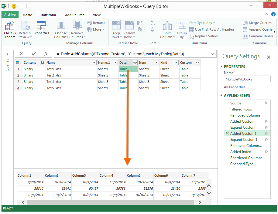
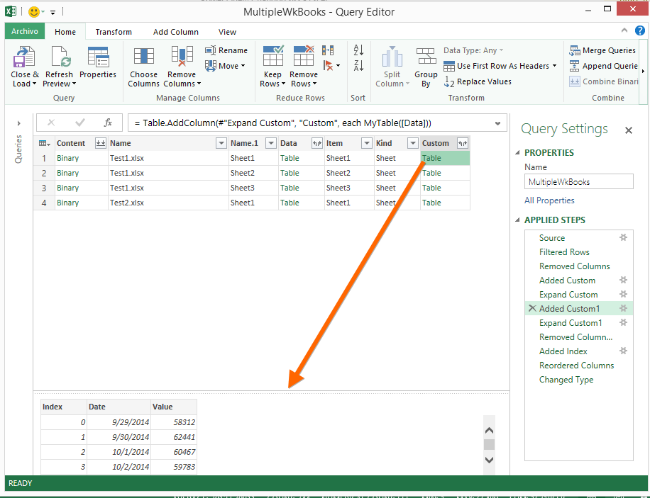
In order to create such column, we are going to apply the function to the Data column (which is a table) like this:

... and we'll get a new Custom column that contains a bunch of Table objects. We can now compare that table from data against the newly created custom column:
Final Steps:
Expand the new column (by clicking that little double headed arrow at the top,) reorder the columns and change the data type, until we have a final table that looks like this:

We're now got a table that is the combination of multiple sheets from multiple workbooks which all went through our transformation, and then were all combined into a single table. All thanks to Power Query.
If you want to see the step by step process then you can check out the video below: