This week we've got a guest post from Miguel Escobar, who is going to tell us why transforming data with Power Query is his first preference versus other tools and methods.  In fact, this is part 1 of 2, and we're going to turn this week over to Miguel in full (I'll be back next week with a new post of my own.

Miguel, the floor is yours!

Transforming data with Power Query

Looking for some cool scenarios to test the power of Power Query in terms of transformation I stumbled upon a really cool post that Chandoo made a few weeks ago where he basically needed this:

(Image taken from Chandoo.org)

He used a really cool formula as option #1 and for option #2 a VBA approach. Now it’s time to make an option #3 that I think will become your #1 option after you finish reading this!

Step #1: Make this a table

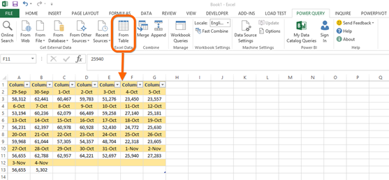
In order for this to work, you’ll need to make the range a table with no headers and that should give you a table like this one:

Also, if you want to follow along, you can download the workbook from here.

Since now we have a table, we can use that as our data source in order to work with Power Query:

(Choose From Table in the Power Query Ribbon)

Step 2: The actual transformation process

Note: Before we start, I don’t want you to be scared of some M code that we’ll be showing you later. Instead, I’m going to show you how NOT to be scared of this crazy looking M code and tell you how it was originated. And no, I didn’t manually go into the advanced editor to do anything – I did all of my steps within the actual UI of Power Query  

So we start with 3 simple steps:

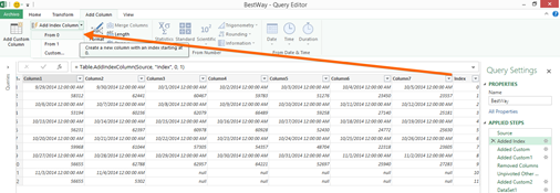
Add an Index column that starts from 0 and has an increment of 1:

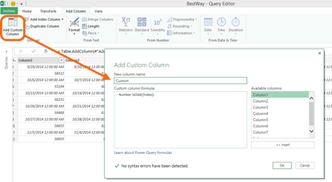
Then we move forward with defining the odd and even rows with a custom column using the Index as a reference and the Number.IsOdd function:

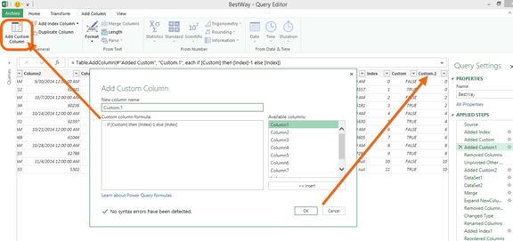
After this, we will create another custom column based on the one we just created with a simple if function;

We can see that our table so far has 3 custom columns:

• Index
  • that starts from 0 and has increments of 1
• A TRUE/FALSE column that tells us if the row is odd or not
  • we used the Number.IsOdd function here
• A column that basically gives the same number for the records in every 2 rows. So essentially we are creating a pair – a couple

The next step would be to remove the Index column as we no longer need it.

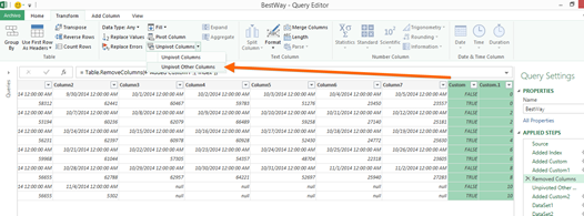
And now select the Custom and Custom.1 columns and hit the unpivot other columns option:

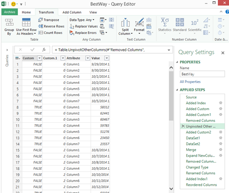
And now our query should look like this:

It's all coming along great so far...

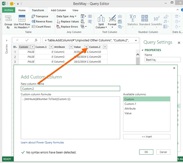
Now we create another custom column that will help us along the way. This will work as our column ID for the components of a row.

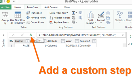
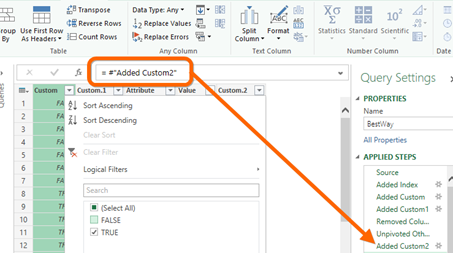
And now here’s where the interesting part comes. You need to hit the Add Step button from the formula bar:

And that should give us a query with the results from the last step which in our case is the “Added Custom 2” step. In this section we will filter the custom column to only give us the rows with the value FALSE.

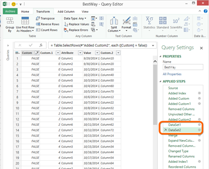
You’ll go back to the “Added Custom 2” step and basically repeat the “Add a custom Step” process but this time you’ll filter it to be TRUE instead of false. I’ve renamed this 2 steps in my query to be DataSet1 and DataSet2.  (Right click the step in the "Applied Steps" box and choose Rename to do this.)

Tip: You can always check what’s going on in a step by hitting the gear icon right next to the step.

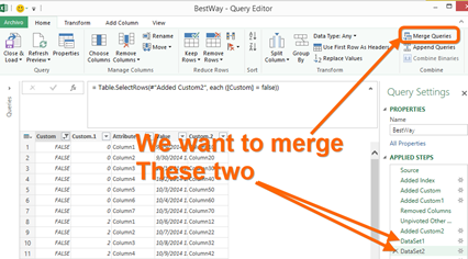
Now we want to combine those 2. DataSet1 and DataSet2....but how?

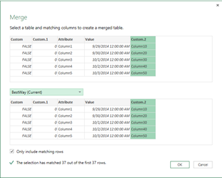
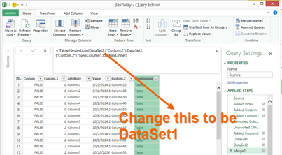
We hit the Merge Queries button but you’ll notice that it will only show you the tables and queries that have been loaded to our workbook or that are stored as connections. So for now we’re going to trick the system and just choose a merge between the tables that PQ tell us to choose from like this:

And that should give you this:

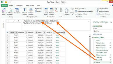
And we need to change what we have in our formula bar in either one of the DataSet2  to be DataSet1 so we can merge the data from DataSet1 and DataSet2 which should give me this:

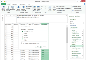
As you can see, we have a column that needs our help. Let’s expand that new column but only the column with the name Value like this:

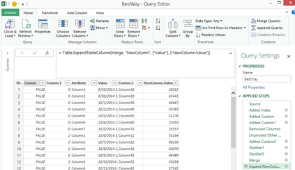
And the result of that should be:

We are almost there

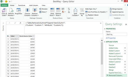
We have the data how we want it, but now we want to clean it as it has some columns that we don’t really need, so just remove the columns using the Remove Columns button from the Power Query UI (User Interface):

This looks more like it! but wait, we need to add some data type and perhaps rename those columns so it can be readable for an end-user.

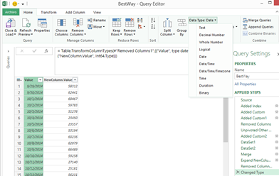
First, we change the data type for both columns as desired:

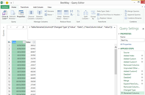
And later we proceed with renaming the columns just by double clicking each column name:

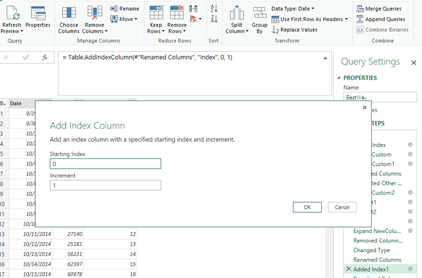
In Chandoo’s solution, he adds an index column for the end result so we’ll do the same:

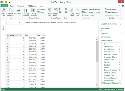
And this is our final result after we reorder our columns just by drag-n-drop:

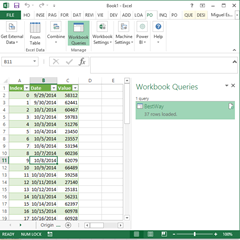
Once its loaded into our Worksheet it’ll look like this

Things to take in consideration

1. This is a dynamic solution. You can add new columns and/or more rows and it will still work as desired.
2. This WILL work on the cloud with Power BI so you can rest-assured that what we just described is something that we can refresh on the cloud. (VBA doesn't work on the cloud.)
3. We could potentially transform this into a function and execute that function into multiple sheets, tables and even defined names within one or multiple workbooks. (Read more about that here.)
4. If the result of this transformation has an extensive amount of rows, we could load it directly into our Data Model instead of experiencing the performance drawback of loading it into a worksheet. (Things get seriously slow when a workbook gets way too many rows.)

Power Query is a tool that was created specifically for scenarios that needed transformation like this one.  Microsoft is on a roll by delivering monthly updates of Power Query and you can bet that it will continue to get better and better each month, as it already has for the past year and a half to date.

Try Power Query if you haven’t done so yet. Download the latest version here