I'm currently hanging out in New Zealand, with a friend who has generously let me stay at his place instead of a hotel. What I didn't know when he offered a bed though, was that the cost of admission was a solution for a gnarly Power Query issue he was facing: How to unpivot stacked sets with inconsistent rows.
The data Jeff provided me with looked similar to this:
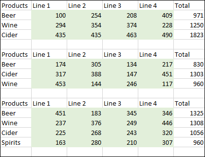
If it were only the first two tables that we were facing, this wouldn't be too difficult. We cover unpivoting stacked data sets in both our Power Query Academy and our Power Query Recipes, whether they are single or multi column. But the killer here is the third table... it has more rows than the first two. So the question becomes how do we unpivot stacked sets with inconsistent rows?
Preparing the Data
Obviously the first piece we need to do is to get the data into Power Query and remove the irrelevant rows and columns. The steps I went through were these:
- Pull the data in to Power Query
- Filter Column1 to remove null values
- Remove the Total column
Once done, my data looked like this:
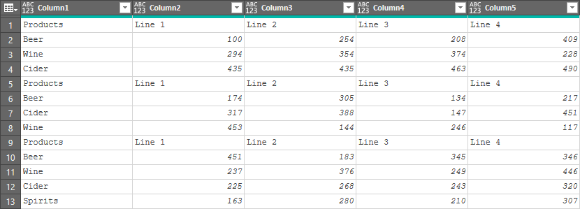
So now the data is nice and clean, but how to you unpivot it?
Separating the Data
The first trick is to find a way to separate this data into individual tables that represent each of the stacked data sets. The good news here is that there is an indicator that we are looking at a new table. Every time we see "Products" in Column 1, we know that's a header row and a new table will begin. So we'll use this to separate the data into blocks, starting a new block each time we see that term. To do this:
- Go to Add Column --> Index Column --> From 1
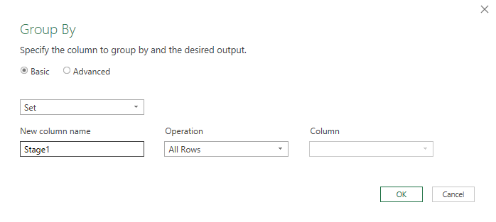
- Go to Add Column --> Conditional Column and configure it as follows:
- Name: Set
- Formula: if [Column1] = Products then [Index] else null
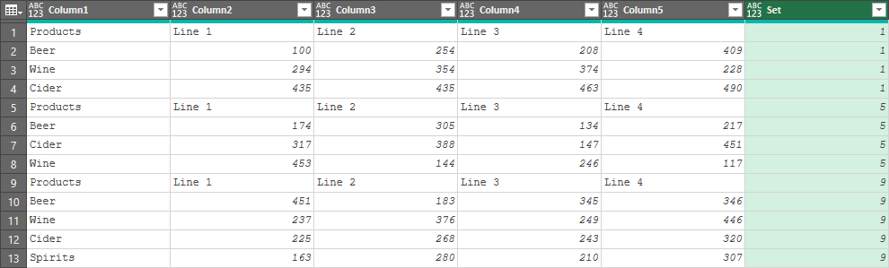
Shown below is the image view of the Conditional Column, as well as the results that it will create:
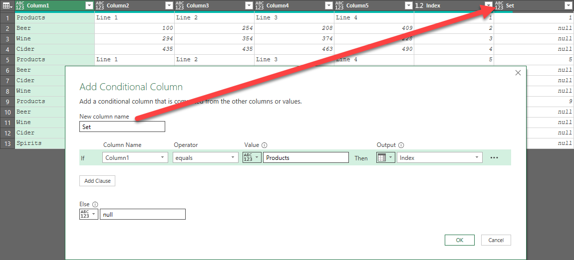
As you can see, we've pulled out the number from the Index column if - and only if - the value in the first column is "Products". The reason we want the null is that we can then:
- Right click the [Set] column --> Fill Down
- Select the [Index] column --> press DEL
You're now left with a nice table where the Set column shows a unique value for each data group:
Grouping Into Tables
With an indicator for each group of data, we can now leverage this to separate the data into the individual data sets. The method to do this is Grouping.
Select the Set column and then:
- Go to Transform --> Group By and configure as follows:
- Group by: Set
- New Column Name: Stage1
- Operation: All Rows
The data will then be grouped by the values in the Set column, and show the original data that was used to generate those groups. Clicking in the whitespace beside the Table keyword will show each of these rows that were used in the grouping for that data point:

Cleaning up the Grouped Tables
The challenge we have here is that we want to unpivot the data, but we've got some extra data here that will pollute the set: the values in the "Set" column which were added to allow the grouping. We need to remove that. To do so:
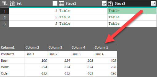
- Go to Add Column --> Custom Column and configure it as follows:
- Name: Stage2
- Formula: =Table.RemoveColumns( [Stage1], "Set"
Compare the results to that of the Stage1 column:
Before we can unpivot data, we need to promote that first row to headers... but we need to do it for each column. No problem, we'll just break out another custom column:
- Go to Add Column --> Custom Column and configure it as follows:
- Name: Stage3
- Formula: =Table.PromoteHeaders( [Stage2], [PromoteAllScalars=true] )
Wait... what? How do you figure that out? I cheated. I grabbed another table, promoted headers, then looked in the formula bar to figure out the syntax I needed. The function name and table name were pretty obvious but unfortunately - even with intellisense - that final PromoteAllScalars part doesn't auto-complete. Even worse, if you don't included it, it essentially just eats the top one row. Once I had it correct, the results are exactly what I needed:
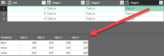
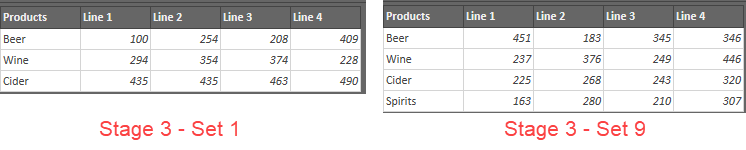
As you can see in the image below, the Stage 3 table contains columns that have headers, as we wanted. The 3rd table (carrying the identifier of Set 9), shows four rows, while the other tables show 3 rows. So the data is now separated into tables, but they still have an inconsistent number of rows.
Unpivot the Data
We have done everything we need to do in order Unpivot Stacked Sets with Inconsistent Rows. We now just need to unpivot the data. So let's do it:
- Go to Add Column --> Custom Column and configure it as follows:
- Name: Stage4
- Formula: =Table.UnpivotOtherColumns( [Stage3], {"Products"}, "Date", "Units" )
An indented version of the formula, as well as the results it produces, is shown here:
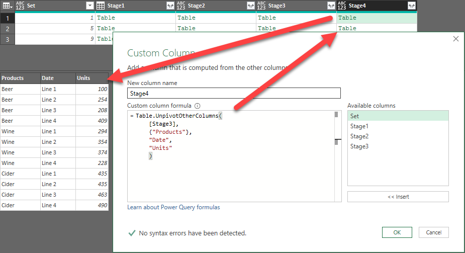
How do you learn to write this? Click on one of tables to drill in to it, unpivot the single table, copy the code from the formula bar, then delete the temporary steps to back up. You may need to do some tweaking, of course, but at least you can easily get the syntax that way.
Now that we have this, we can finish extracting the data:
- Right click the Stage4 column --> Remove Other Columns
- Click the Expand icon at the top of the Stage4 column
- Set the data types
- Load it to your destination
Sample File
If you'd like to download the sample file, you can do so here.
15 thoughts on “Unpivot Stacked Sets with Inconsistent Rows”
Am I allowed to delete the blank rows and the duplicate header rows in Excel first? If so, it becomes a trivial PQ unpivot.
If not, I can pull the data into PQ, remove empty rows, filter out rows with "Products" in the first column (I didn't have to promote the first row to column headers, it just happened). Then unpivot.
Or have I oversimplified the process?
Hey Jon,
Actually, I oversimplified the data set in order to shoot narrower images. Originally, the headers were dates with each header increasing by a week (so they weren’t the same). I lost that nuance when I changed up the data. Doh!
Hopefully that makes more sense!
Ken just got tired of looking up my date all week.
Hello there is an errata the 'Unpivot the Data' section,
It reads:
Go to Add Column --> Custom Column and configure it as follows:
Name: Stage3
Formula: =Table.UnpivotOtherColumns( [Stage3], {"Products"}, "Date", "Units" )
Should be.
"Name: Stage4"
Thanks Fernando, I've updated it. Cheers!
I looked at this problem and thought, so many steps? Why? Then I did it my way and my M Code is 16 lines long yet yours is >30 lines long and relatively complex, or so. As Jon Peltier says, it's trivial.
Then I saw your response to Jon's comment ... I will rework this exercise taking that into account!
I reworked that, thanks again Ken. It worked a treat!
Can I point out that in the section headed Cleaning up the Grouped Tables,
This Formula: ... needs a closing parenthesis:
=Table.RemoveColumns( [Stage1], "Set"
Hi Ken,
I have the same thoughts as Jon. I don't quite get it...
Do you mean the headers should be something like Week 1, Week 2, in table 1, Week 5, Week 6... in table 2, and so on?
Nevertheless, here's my attempt to get the same result using your sample workbook. Appreciate your comment.
let
Source = Excel.CurrentWorkbook(),
#"Filtered Rows" = Table.SelectRows(Source, each ([Name] "OutputQuery")),
Content = Table.Combine(#"Filtered Rows"[Content]),
#"Removed Columns" = Table.RemoveColumns(Content,{"Total"}),
#"Unpivoted Other Columns" = Table.UnpivotOtherColumns(#"Removed Columns", {"Products"}, "Date", "Value"),
#"Changed Type" = Table.TransformColumnTypes(#"Unpivoted Other Columns",{{"Products", type text}, {"Value", Int64.Type}})
in
#"Changed Type"
Hi Ken,
If you don't mind, I would like to share my video talking a similar situation of un-stacking uneven data with Power Query.
https://youtu.be/YInCL1yNxNc
Hope you like it.
Cheers,
Reading the comments, I replaced the word 'Products' with random dates. Then I came up with the following:
let
Source = Excel.CurrentWorkbook(){[Name="BeforeData"]}[Content],
#"Get Date from column 1" = Table.AddColumn(Source, "Date", each Date.From([Column1])),
#"replace Error with null" = Table.ReplaceErrorValues(#"Get Date from column 1",{{"Date",null}}),
#"Filled Down Dates" = Table.FillDown(#"replace Error with null",{"Date"}),
#"Promoted Headers" = Table.PromoteHeaders(#"Filled Down Dates", [PromoteAllScalars=true]),
#"remove nulls and subsequent headings" = Table.SelectRows(#"Promoted Headers", each ([Line 1] null and [Line 1] "Line 1")),
#"Renamed Columns" = Table.RenameColumns(#"remove nulls and subsequent headings",{{"2/2/2020_1", "Date"}}),
#"Changed Type" = Table.TransformColumnTypes(#"Renamed Columns",{{"Line 1", Int64.Type}, {"Line 2", Int64.Type}, {"Line 3", Int64.Type}, {"Line 4", Int64.Type}, {"Total", Int64.Type}, {"Date", type date}, {"2/2/2020", type text}}),
#"Reordered Columns" = Table.ReorderColumns(#"Changed Type",{"Date", "2/2/2020", "Line 1", "Line 2", "Line 3", "Line 4", "Total"}),
#"Removed Columns" = Table.RemoveColumns(#"Reordered Columns",{"Total"}),
#"Unpivoted Other Columns" = Table.UnpivotOtherColumns(#"Removed Columns", {"Date", "2/2/2020"}, "Attribute", "Value")
in
#"Unpivoted Other Columns"
Note: I cheated a little because my version of PQ didn't have Table.ReplaceErrorValues as a choice so I keyed it in.
Thanks Ken. Great solution, as always.
While I was replicating the steps I realised that adding Stage 4 may not be necessary as the column names are already identical in all 3 sets. So, Stage 3 can already be expanded. However, if your had or anticipate to have different 'Line #' column names across the sets adding Stage 4 step becomes more justifiable.
Assuming Line1,Line2 etc are End of Week Dates that increase with each "block"
let
Source = Excel.CurrentWorkbook(){[Name="D"]}[Content],
mAddIndex = Table.AddIndexColumn(Source, "Index", 1, 1),
mAddCol = Table.AddColumn(mAddIndex, "Custom", each if [Column1]=null then [Index] else null),
mFillUp = Table.FillUp(mAddCol,{"Custom"}),
mFilterOutNull = Table.SelectRows(mFillUp, each ([Column1] < > null)),
mRemCols = Table.RemoveColumns(mFilterOutNull,{"Index"}),
mCombine = Table.Combine(Table.Group(mRemCols, {"Custom"}, {{"GRP", each Table.SelectRows(Table.UnpivotOtherColumns(Table.PromoteHeaders(Table.RemoveColumns(_,{"Custom"})),{"Products"},"WeekNo","Amt"),each [WeekNo] <> "Total"), type table}})[GRP])
in
mCombine
Thanks Sam. Fixed up the code for the eaten gt & lt symbols too. 🙂
@Ken - you missed out the below
mFilterOutNull = Table.SelectRows(mFillUp, each ([Column1] n.e. null)),
Thanks
Sam
Done. 🙂