In my last post, I looked at how to pull a named range into Power Query and turn it into a table of data.  Today we’re going to look at how to create dynamic table headers with Power Query, but using a slightly different, slightly more complicated way to do the same task.  Why?  Well, the reality is that sometimes the simple method won’t work for us.

Background

In this scenario, we’re going to use the same file I used in my last post, we’re just going to build the output differently.  The key that I’m after here is that I want to pull the data range into Power Query, but I want to use a table.  The issue, however, as I mentioned in my last post, is:

If I set up the table with headers in row 3, it would convert the dates to hard numbers, thereby blowing apart the ability to easily update the dynamic column headers next year.  That would defeat the purpose of making the input sheet dynamic in the first place.

I’ve really struggled with this feature in Tables, where it converts your headers to hard values.  So many of the tabular setups I create use dynamic headers, it’s actually more rare that they don’t.  So how do we work around this?  How do we create dynamic table headers in Excel?

Setting Up The Table For Success

It’s actually a LOT easier than you might think.  I use this very simple trick with both PivotTables and regular Tables, allowing me to take advantage of their power, but still control my headers and make them dynamic.  Here’s how:

Step 1: Add Static Headers Manually

• Insert 2 rows below the current dynamic date headers in Row 3
• Put some static headers in Row 5 that are generic but descriptive.  (In this case, CYM# means “Current Year, Month #”)

The important part here is to make sure these static headers are each unique so that you can “unwind” them later with Power Query.

Step 2: Create The Table

Next, we need to create the table.  It’s going to cover A5:N24, and will therefore inherit the CYM column headers.  Since they are static values, it won’t make any changes to them, and my dynamic dates are still showing up top.

Step 3: Build a Translation Table

Huh?  A what?  Bear with me, as this will come clear a bit later.  Here’s how we do it:

• Enter the following in B4:  =B3
• Copy this across to cover B4:N4
• Make sure B4:M4 is selected and go to Home—>Editing—>Find & Select –> Replace
• Using the dialog, make the following two replacements:
  • Replace = with =$
  • Replace 3 with $3

This has the effect of making the formulas all absolute, which is important for our next step.

• Select B4:N5 –> Right Click –> Copy
• Select a cell down below your data range somewhere (I used A34)
• Right click the cell and choose Paste Special
• In the Paste Special options, choose the following:
  • Paste:  All
  • Check the Transpose box

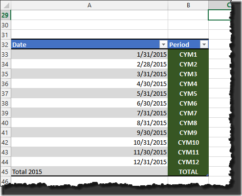
Very cool, we’ve now got the beginnings of a table that is linked to the formulas in row 3.  We just need to finish it.

• Add the column header of “Date” in A33
• Add the column header of “Period” in B33
• Format the data range from A33:B46 as a table
• Rename the table to “DateTranslation”

Step 4: Final Header Cleanup

Row 4 has now served it’s purpose for us, so you can delete that, and then hide (the new) row 4.  The end result is that we have a header on our table that looks like it’s part of the table, but isn’t really.  The benefits here are that we can preserve the dynamic nature of it, and we have a wider variety of formatting options. We also have a completely separate date translation table too…

Setting Up The Power Query Scripts

So now we need to get the data into Power Query.  Let’s do that.

Step 1: Import and Reformat the Rounds Table

To do this we will:

• Click somewhere in the main table
• Power Query –> From Table
• Remove the “TOTAL” column
• Filter the first column to remove text that begins with “Total” and values that equal null
• Filter the second column to remove null values
• Right click the first column and Un-Pivot Other Columns
• Rename the “Month” column to “Round Type”
• Rename the query to “Budget”

At this point, you should have the following: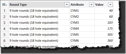

This is great, but what about the Attribute column.  This is the whole big pain here about using a table, in that we don’t have dates.  Yes we could have hard coded them, but then it would be very painful to update our query when our year changes.  So while we have something flexible (in a way) here, it isn’t really all that readable.  How can we change that? Save and close the query, and let’s deal with this.

Step 2: Create Another Power Query

Let’s add the other table we built:

• Click inside the DateTranslation table we created
• Go to Power Query –> From Table
• Click Close & Load –> Load To…
• Click Only Create Connection –> Load

This will create a new Power Query that basically just reads your original table on demand.  It won’t refresh unless it’s called from another source.  Now we’re set to do something interesting.

Step 3: Re-Open The Budget Power Query

If the Workbook Queries pane isn’t open on the right, then go to Power Query –> Workbook Queries to show it.

• Right click the Budget query and click Edit
• On the Power Query Home tab, click Merge Queries (in the Combine group)
• Select the Attribute column
• From the drop down box, choose Date Translation
• Select the Period column
• Make sure “Only Include Matching Rows” is checked and click OK

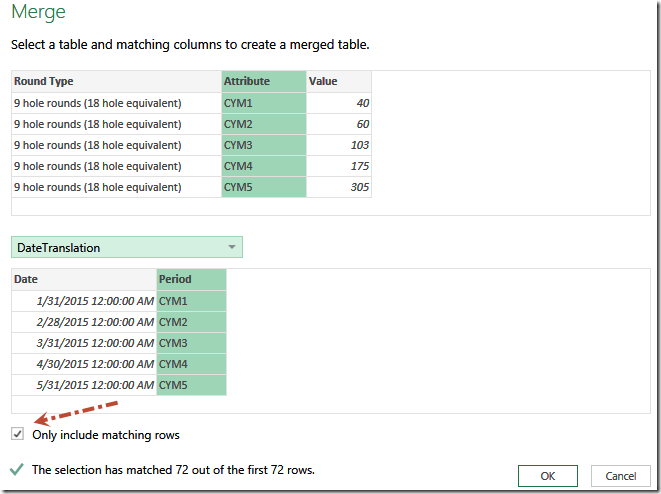At this point you’ll get a new column of data in your Query.  Click the icon in the top right of the column to expand it:

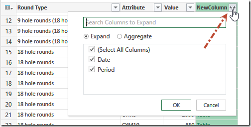
Excellent… now we only need to pick the column we need, which is Date.  So uncheck the Period column and click OK. Finally we can remove the Attribute column and rename the “NewColumn.Date” column to Date and we’ve got a pretty clean query: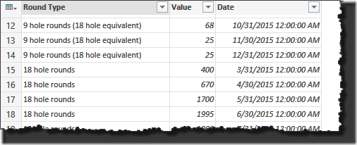

At this point we could call it a day, as we’ve pretty much accomplished the original goal.  I can update the Year cell in B1 and my Table’s “Headers” will update.  In addition, my Power Query will show the correct values for the dates as well.  Pretty cool, as I could now link this into Power Pivot and set a relationship against a calendar table without having to worry about how it would be updated.

Going One Level Deeper

One thing I don’t like about this setup is the need for the extra query.  That just seems messy, and I’d prefer to see just one query in my workbook.  The issue though, is that I’m pulling data from two tables.  What’s cool though, is that with a little editing of the M code, I can fix that. Here’s the M for the query I’ve built, with a key line highlighted (twice): As you can see, the “Merge” line is coloured yellow, but the name of the Query being merged is in orange.  Well guess what, we don’t need to reach to an external query here, we can reach to another named step in M.  Try this: Immediately after the “Let” line, enter the following:

TranslationTable = Excel.CurrentWorkbook(){[Name="DateTranslation"]}[Content],

Now, modify the “Merge” line to update the name of the table from “DateTranslation” to “TranslationTable”.  (The reason we’re doing this is that the original query still exists, so we can’t just name the first step “DateTranslation”, as it will conflict. Once we’ve made our modifications, the script will look as follows: When you click “Done”, the query will reload and you’ll see an extra step in the “Applied Steps” box on the right.  What you won’t see though, are any changes, as the data comes out the same.  Very cool, as we are now referencing both tables in a single step.  To prove this out, save this query, drop back to Excel and delete the “DateTranslation” query.  It will still work! (The completed file can be downloaded here.)

Ending Thoughts

I really like this technique.  It let’s me dynamically change the column names, yet still use those to link them into my data model tables.  But even more I like the ability that, with a minor edit to the M code, I can keep my workbook from being littered with extra queries.  🙂