One of the methods we use when building business solutions is creating specific input sheets for our models, as it separates our data from our business logic and ultimately our reporting layers.  This strategy is a key piece of building stable models, and is one of the fundamental things I teach when I’m leading modelling courses.  (For more information on having me at your site, click here.)  Since many data entry points consist of non-contiguous ranges in Excel, it make sense to look at how using non-contiguous data ranges in Power Query can help us in our modelling.

To that end, in today’s blog post, I’m going to look at a technique to take a standard data entry worksheet and turn it into a data source, which can then be linked in to the model (or just used as the basis of reports.)  This is ideal, as we then only have one place to update our data for our solution.

Background:

What we’re going to start with is this:

A few key things you might want to know are:

• You can download the sample file from this link if you want to follow along.
• This is hypothetical budget data for golf rounds.
• All the data entry cells are light green (I tell my users “Green means go” and they are now conditioned to stay away from anything that isn’t that light green colour.
• The year in cell B1, when changed, will update all of the headers on the input sheet to the current year

Now, what I’d like to do is un-pivot this data into a useable table.  If I could do that, then I’d be able to use it in any of many methods, such as PivotTable, PivotCharts, charts or VLOOKUP solutions.

The initial setup

Your first temptation might be to layer a table over the data.  I’ve got a few reasons why I don’t want to do that:

1. If I did layer a table over my input form it would lose the intuitive “enter data here” setup that I worked so hard to create.  Users would end up with a banded table that didn’t indicate where data should go.  That’s not ideal.
2. If I set up the table with headers in row 3, it would convert the dates to hard numbers, thereby blowing apart the ability to easily update the dynamic column headers next year.  That would defeat the purpose of making the input sheet dynamic in the first place.
3. If I set up the table with headers above that, I’d end up with a bunch of ugly Column1, Column2 headers.  I suppose I could hide them, but again, my table would blow apart my formatting as mentioned in 1.

So no… that’s not what I’m after.  So now what…?

There’s actually a few different ways to handle this.  I’ll look at some others in later blog posts, but for now let’s piggyback on the technique about using named ranges that I covered in my last post.

Creating the Named Range

The first thing I’m going to do is create a named range (not a Table) to cover the entire range that holds my budget data: A3:N22.  That includes the headers, all blank rows ,and all data right up to the totals on the right and bottom.  The reason for this is that, should I end up adding any new categories later by inserting rows or columns, it’s fairly likely that I’ll be doing it before the totals, so they’ll get picked up.  (It’s not quite the auto-expansion feature of a table, but it’s the best I’m going to get with a named range.)

So I created my named range and give it a sensible name like rngBudgetData.

Pulling the data into Power Query

Now let’s look at the easiest way to get our named range into Power Query.

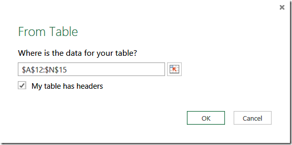
If we click a single cell in our data range, then told Power Query to get the data from a Table, we’d be given a range for that expanded to cover only the contiguous block of data.  Because we’ve got blank rows in our data, that wouldn’t really work for us.  For example, assume we click B3, then tell Power Query to pull data From Table.  We’d be given the range A12:N15, as shown below.

Alternately, we could create a blank query, then type =Excel.CurrentWorkbook() in the formula bar, and choose our table, as outlined in the last blog post:

Okay, so that WOULD work.  As it turns out though, there is still yet another way to do this:

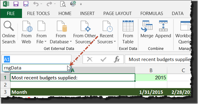
• From the Name drop down in Excel, select the rngBudgetData named range

• A3:N22 will now be selected, so go to Power Query –> From Table

And look at that, we’re now in Power Query using our named range!

The secret to this is, in order for Power Query to pull in the named range, the entire named range must be selected.  If that happens, Excel will grab it as the Power Query source.  If you’re using named ranges that cover contiguous blocks of data, and you click somewhere in that block of data, then Power Query very well may grab your entire named range.  So long as the auto selection boundaries line up with your named range you should be good.  But in the case of my data, those blank rows blow that apart, which is why I selected it from the name drop-down first.

(It is worth noting that if a named range and a table’s boundaries match exactly, the Table will be used as the Power Query source, not the named range.)

Manipulating the data in Power Query – Issue 1

Upon pulling the data into Power Query, we end up with a table like this:

Naturally, the first thing we want to do is promote the first row to headers, so that we can get to un-pivoting the data.  But look what happens when we do:

What the heck?  The first column was renamed to Month (from the first row of data), but the remaining didn’t change! Not only that, but we lost our date time stamp.  That’s not good.

So it appears that Power Query can’t promote a date/time into a column header.  We’d better remove that step and try another approach.

Removing Irrelevant Data – Cut 1

Before I get into dealing with the harder stuff, I’m going to do a quick bit of cleanup here.  I’ve got some bank rows of data in my table, so I’m going to knock those off first.  To do that I:

• Filter Column1 and uncheck (null) values

I’ve also got some header rows, which I can identify by the null values in Column2-Column14.  I can knock those off as follows:

• Filter Column2 and uncheck (null) values

Easy enough so far.  I also don’t need the Total column, so I’ll scroll all the way to the right and:

• Right click Column14
• Choose Remove

Now I need to get rid of all the rows that contain totals (as I can always re-create those with a Pivot Table:

• Filter Column1
• Text Filters –> Does Not Contain –> “Total “ –> OK

Now, you’ll notice that I used Total with a space.  This is just to make sure that I don’t accidentally remove a row that contains a word which has total in it – like “totally”.  It’s always safer to make your text pattern as exact as possible.

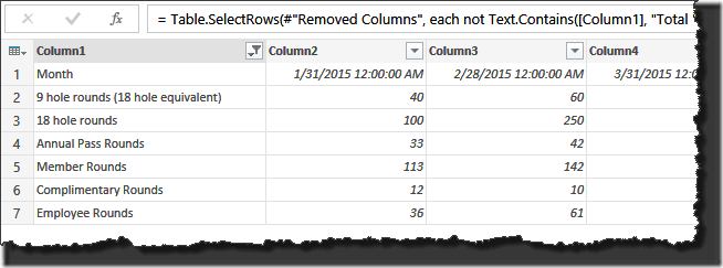
After doing all of the above, I’m left with this:

So the data is all clean, but I still can’t promote my headers so I can un-pivot this data.  Now what?

Busting Out Transpose

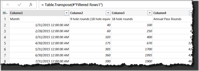
Transpose is quickly becoming one of my favourite functions.  Let’s hit it now:

Hmm… originally I was going to convert my dates to text, Transpose it back, promote the text to headers, then un-pivot it.  But I don’t think I even need to do that at all.  Try this:

• Transform –> Use First Row as Headers
• Select the Month column
• Transform –> Unpivot Columns –> Unpivot Other Columns

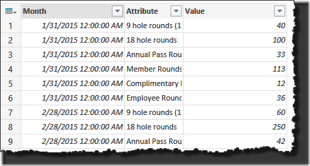
Bingo!

Now just for the final cleanup:

• Select the Month column –> Transform –> Data Type –> Date  (You need to do this, or Excel will return date serial numbers to the table, not dates formatted as dates.)
• Rename the Attribute column to “Round Type”
• Rename the Value column to “Amount”

Finally we can choose to Close and Load the Power Query and it will turn it into a nice Excel table.

Some Thoughts

As I was developing this blog post I found about 10 different ways through this process to end up at the same goal.  This is actually one of the things I enjoy about Power Query is the creativity that you can employ coming out to the same end result.

One feature I do hope to see eventually is the ability to filter for text that “starts with” or “does not start with”.  That would allow me to make my text searches even tighter than the “contains” portion I used here.  In one version I actually wrote an if function to do that:

=if Text.Start([Column1],5)=”Total’ then “remove” else “keep”

The loss of the months when originally promoting the header row shocked me a bit.  I would have expected this to be automatically converted to text and those values used.  Alas that’s not the case, so we have to do a bit more work.  Certainly not the end of the world, but not what I’d expect to see.

At the end of the day though, it’s nice to know that there is a way to get useful non-Table data into Power Query and turn it into something useful.  🙂