Making an Icon Set show only two conditions

2009-04-23
Ken Puls
Categories: Excel

I really like the new icon sets that are in Excel 2007. They're kind of a neat way to format a cell to show interpretive information at a glance.

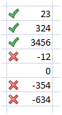
One practical place to use these is as an alternative to the using custom number formats that I blogged about last year. I decided to use Excel's icon sets to show a green check when something was positive and a red x when negative, as shown below:

One thing that can be frustrating when trying to set this up is that Excel forces you to use the three part icon set. By default, the image above would have a yellow exclamation beside the zero. Personally, I don't need it. But with Excel forcing it on you, how do you avoid it? Here's how I did it:

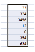
Select the cells:
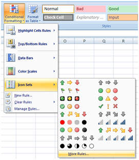
From the Home tab, choose Conditional FormattingÃ Icon SetsÃ More Rules
Using the default of "Format All Cells Based On Their Values", set up the rule as follows:
You'll need to change:
- The "Type" fields to "Number"
- The Icon Style
Apply the rule

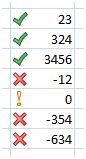
Now you have the cells looking as shown below, but how do you hide the yellow exclamation on the zero?

The answer is to set up a conditional format using another of Excel 2007's conditional format tools; Stop if True

Select the cells again
This time choose "New Rule" from the Conditional Formatting menu (not "More Rules" from the icon set area)
Choose to "Format only cells that contain" and set up the rule as shown below:

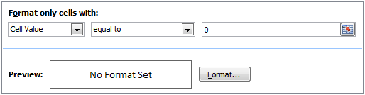
Applying the rule now won't have any effect, as it is essentially a blank rule. (See the message about "No Format Set"?)

Click Format
On the "Fill" tab, click "No Color" for the background and click OK twice

We now have our second rule set up, but nothing appears different. Let's fix that:

With the cells still selected, go back and choose "Manage Rules" from the Conditional Formatting menu
Check the "Stop if True" box beside your latest rule as shown:

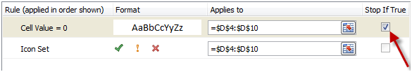
Click Apply and it should the yellow exclamation disappears from the scenario.

The "Stop if True" feature is a great addition to Excel's conditional formatting as it allows us to decide just how many of our formats we wish to overlay in 2007. Depending on how many you apply to one cell though, you may have issues with trying to figure out inheritance issues, so use them carefully.

11 thoughts on “Making an Icon Set show only two conditions”

xluser2003 on June 1, 2009 at 5:12 pm said:

Hi Ken,

Is there any equivalent version of this great hint for Excel 2003, or can it be replicated with VBA?
Ken Puls on June 4, 2009 at 7:35 am said:

Hi there,

Debra Dalgleish wrote up an article on making icon sets in 2003: http://blog.contextures.com/archives/2009/04/14/conditional-formatting-icons-in-excel-2003/

Cheers,

Ken
Geoff Conley on June 5, 2009 at 6:17 am said:

I am trying to do the two conditions but the first is to highlight cells that are unlocked, but then remove the highlight when data is entered. I'm trying to create a template for labels, and trying to make it easy for the non exp user to know what boxes they can type in.

Thanks

Geoff
Ken Puls on June 5, 2009 at 6:29 am said:

Hi Geoff,

You actually only need one condition. Set up your rule with the following formula (assuming the cell is A1):

=Len(A1)=0

Set the format to the colour you want.

At this point it should highlight any cell that has no data in it. Put something in and the colour will go away.
Geoff Conley on June 9, 2009 at 7:11 am said:

Ken,

That works but the problem is not with all tha highlighted that will print onto the labels we are using. Is there anyway to combine the len statement so that it will work with the Cell statement?

Thanks
Ken Puls on June 9, 2009 at 7:16 am said:

Not sure I quiet followed that...

So you want to hide any remaining conditional formats before you print? You could have a look at https://excelguru.ca/2009/05/11/trigger-conditional-formats-before-printing/

To make that work you'd end up with a formula like:
=AND(Len(A1)=0,rngPrintMode="Yes")

I haven't actually tried to evaluate this using at CELL statement personally.
Geoff Conley on June 9, 2009 at 7:29 am said:

Is there anyway i can upload you the file so that you can see what I'm trying to do? Basically i want only the unprotected cells to fill a color when empty but when data is entered the fill is removed.
Reed Jacobson on July 26, 2009 at 12:33 pm said:

Hi Ken,

If you're willing to let the zero cell have a green check, you can just set both the green check and the yellow bang conditions to >= 0. The yellow one won't ever get hit.

What I'm trying to find is a way to have two icon-set rules that get applied based on formula. For "cash inflow" accounts I want the default arrow icons. For "cash outflow" accounts I want them with reversed order. The UI doesn't allow you to put a formula and then use an Icon Set. The object model SAYS there's a Formula property for the IconSetCondition object (and Excel Help even says it works), but I just get an error. Have you played with this at all?

(I'm also totally annoyed that the new formatting can only use the value from the current cell as the base value. I really want it to be the result of a formula. If it were a formula, I could achieve my objective by having the formula secretly invert the values of the "cash outflow" accounts. But using a formula for the value doesn't appear to be even ostensibly possible.)

Nice blog. I'll have to bookmark you.

Cheers,
Reed
Ken Puls on July 27, 2009 at 8:50 pm said:

Hi Reed,

When you're setting up your icon set, change the "Type" to Formula from "Percent", and you should be able to do what you're after.

You're right that you can't use a formula in a conditional format and do anything to blank cells, but you could always use a helper column to coerce your values the right way, then conditionally format that with the formula. (In my experience, it does work.)

Of course, if you can coerce your values using a formula to put it in a cell, you could do so in the formula for the conditional format anyway, so the helper column may not be necessary.
Mark on January 16, 2012 at 5:30 am said:

I am trying to be able to place a geen check, red "x", or a yellow "!" in a cell by either typing Y for green N for no or C for "!". Is there a way to format a cell like this?
J.-P. Pascoli on March 18, 2012 at 5:52 pm said:

Hello. Do you know of any way to get addtional icon sets into Excel 2007, or how to modify existing ones? The problem I have is that I want to use a Green Down Arrow for conditional formatting (for the condition when a value drops - which is a 'good' change) but there is only a Grey Down Arrow available.

J.-P.