I recently taught a course and, while this wasn't actually covered in the course content, we did discuss it. I've found that every time I demonstrate this technique, it gets some "oohs" and "aahs", so I figured that I'd share it here.
The question I was posed is, "I have a spreadsheet where the data is set up across rows, and I'd like it down the columns. Is there an easy way to do that?"
It is a fairly common request, in my experience. One specific example I remember helping a friend with was a list of product and serial numbers that they pulled from a system. I'll pretend that it looked a little like this:
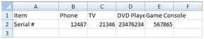
In this case he wanted to change it to a column of item descriptions and serial numbers. It was a lot more columns of course, and was floored when I sent it back to him within a minute. (It took longer to open the file and respond to the email than to fix it.) Here's how you do it:
- Select the data in A1:E2
- Right click and choose "Copy"
- Click in another cell (I chose A5)
- Right click and choose Paste Special
-
In the dialog box shown below, ensure you check "Transpose"
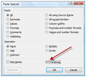
- Click OK and you're done
The completed data looks as shown below:
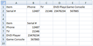
And yes, if you want to go from columns to rows, it works too. Same steps exactly.
4 thoughts on “Turn Data on its Ear”
Ken,
This is a trick I was going to show at the last UK Excel Cnference, but Roger Govier had the same idae and hsi session came first.
If you have a cross-tab type report in Excel, you can transform it to a de-normalised list (which is good for pivotting) like this
Menu>Data>PivotTable and PivotChart Report
Select the Multiple consolidation ranges option
Next
Select the option to create the page fields yourself
Next
Select the source table (or that part of) to be changed, and click the Add button
Next
Pick a location for the pivot table, AND THEN click the Layout button
In this dialog drag both of the Column and Row buttons out of the pivot schematic, leaving just the 'Sum of Value' data field
OK
Finish
This should create a single item pivot
Double-click the cell that contains this single item total, and Excel will create a new sheet with the original data in a flatfile form
Change the column headings to something more meaningful
Hey cool! That's really slick. So you can essentially take a data that's already been laid out in a somewhat pivoted format, and actually get it into a PivotTable compliant structure. Nice!
One question though... where the heck is "multiple consolidations" in 2007? Am I just blind? I can't seem to locate it...
That is true, what a load of cr#p! As you know I am not a 2007 fan, I still use 2003, and that tip was 2003 based.
But ... you can still do it in 2007. Instead of using Insert>PivotTable, use the shortcut keys Alt-D, Alt-P. That will open up the old wizard.
Unfortunately, when you get to step 8, the Layout button is disabled, so you end up not creating a single element pivot as described.
But, you can still do it as you just drag off the row and column elements from the full pivot to get to a single item pivot that you can then double-click.
The thinking of the bright-spark that did that to pivots is somewhat difficult to comprehend (drongo jumps to mind).
That's a neat trick Bob.
I used some code that Colo has on his site for more complex transforms, I used to use it a lot but not so much now.