Last week I posted a technique to show how to calculate a rolling 12 months in Power Query.  One of the techniques used was to refer to other steps during the construction of that query.  Shortly after publishing that, a user asked a question on a non-related post that can make use of the same technique.  Because of this I thought I should focus on that specific technique this week, and where it can add more value.

The Question

I have a data sheet where the generated date shows up in a single cell up on the top and then the data table itself follows.

I created a query to just pick up the generated data but now I want to use that date within a formula of a new column in the 2nd query (the one that pulls/transforms the data table itself). How can I do that?

Now, the asker is working between two queries.  I’m actually not going to do that at all, rather focusing on getting things working in a single query.

The Mock-up

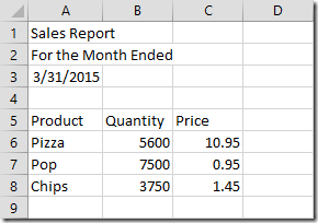
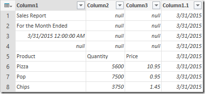
I haven’t seen the asker’s original data, but I mocked up a sample which I believe should be somewhat representative of what was described:

As you can see, we’ve got a single cell with the data in A3, and a table below it.  While I’ve done this in Excel, this could easily be pulled in from a text file, web page, or some other medium. The key that I want to focus on here is how to get that date lined up with the rest of the rows in the table.

Options, Options, and more Options

There’s actually a ton of ways to do this.  Just some include:

• Naming the date range, using the fnGetParameter function to pull it in, and pass it into the query that way.
• Pull the data into Power Query, duplicate the first column, format it as a date, replace errors with null, fill down, and cull out the rest of the garbage rows
• Add a custom column that refers directly the the 3rd field of the first column
• And many more

But in order to pull this of today, I’m going to refer to other steps in the Applied Steps section of the query.  This is a method you can use to determine a variable through the user interface without resorting directly to M code.

Building the Output

Loading the data

To pull the data in, I’ll set up a named range, as this doesn’t exactly look like a table.  To do that I:

• Selected A1:C8
• Replaced the A1 in the Name box (just to the left of the formula bar) with the name “Data”

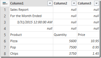
Which landed me the following in Power Query:

Filter down to just the date cell

This part is relatively easy, we just need to:

• Right click Column1 –> Remove other columns
• Right click Column1 –> Change Type –> Date
• Go to Home –> Remove Errors
• Filter Column1 –> Uncheck the null values

And we’re now down to just our date:

You’ll also notice, on the right side, the Applied Steps window shows this step as “Filtered Rows”.  I’m going to right click that and rename it to “ReportDate” (with no space).

Refer to Prior Steps

With this in place, we can now essentially revert to our original query.  To do that, we:

• Go to the Formula Bar and click the fx logo to get a new query line:

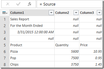
Notice that it refers to the previous step.  No big deal, change that back to “=Source” (the original step of our query.  When you do, your “Custom1” step will look like this:

Perfect.  Let’s add a custom column.

• Go to Add Column –> Add Custom Column
• Set up the custom column as follows:
  • Name:  Date
  • Formula:  =ReportDate

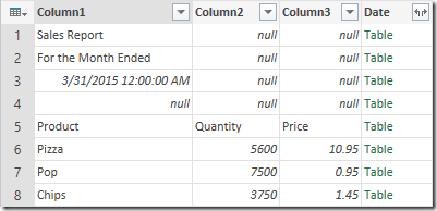
Your “ReportDate” step gets added as a table:

• Click the expand arrow to the top right of the date column header and expand it (without keeping the column prefix)

And now it’s just basic cleanup to get things in the right place:

• Go to Home –> Remove Rows –> Remove Top Rows –> 4
• Go to Transform –> Use First Row as Headers
• Right click Column4 –> Rename –> Date

And you’re done:

So… could you build one query to get the date, then try to pass it to a query with your data table in it?  Sure, but why?  Much better to do it all in one place.

It’s Faster with M

Before Bill S jumps in and shows us that it’s faster when we manipulate the M code directly, I figure I’ll cover that too.  Bill is absolutely correct when he comments on my posts showing why we should learn M.  Here’s the (summarized) route to do the same thing using M code:

• Load the initial table into Power Query
• Go to Home –> Remove Rows –> Remove Top Rows –> 4
• Go to Transform –> Use First Row as Headers
• Add a custom column
  • Name:   Date
  • Formula:  =Date.From(Source[Column1]{2})

You’re done.  🙂

Why?  The trick is all in the formula.  Let’s build it up gradually.

We start by referring to the Source step.

• =Source

This would return a table to the column (as you saw earlier).  We then modify the formula and append [Column1] to this so that we have:

• =Source[Column1]

This returns the list of all of the values in Column1 from the Source step.  (Never mind that we moved past that step – it will still refer to it as if it was still around.)  Next we append the index of the data point we want.  Remembering that Power Query is base 0, that means that we need #2 to get to the 3rd data point:

• =Source[Column1]{2}

Now, if you went with this as your formula you’d find that it actually returns a DateTime value.  So the last step is to wrap it in a formula to extract just the date:

• =Date.From(Source[Column1]{2})

Final Thoughts

So now you’ve seen two ways to pull this off… one via the user interface, one more efficient by writing a small bit of M code.  Different options for different comfort levels.

What I love about Power Query is that you don’t NEED to master M to use it effectively.  But if you DO master M, then it sure can make your queries more efficient and elegant.

Also, I should mention this… if the user really DID want to merge these two queries together, it is as easy as adding a new step (by clicking that fx button), then putting in the name of the other query.  That will bring the data over, and then it’s simply a matter of following the rest of this post to stitch them together.