A couple of weeks ago, Rudi asked how you would go about setting up a query to remove all rows up to a specific value. Specifically, his question was this:
The other day I was asked if Power Query could delete all top rows up to a found value. I could not find a solution and its been a burning question till now.
For example: If I import a csv file containing columnar info, but the headings for the list are in different rows for each import. I know that the first heading in column A is called "ID Number", but each import has this heading in a different row.
How do I determine an applied step to delete all rows above "ID Number". I cannot use the delete top rows as its not always 5 rows, some import the headings start in row 10, others in row 3...but the label I am looking for is always "ID Number".
While the question was answered in the initial post, I still though it would be interesting to do a full post on this for others who might need to create similar functionality.
The Data Set
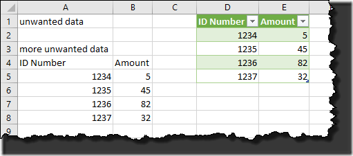
I didn’t have Rudi’s exact data, so I knocked up a little sample with an ID Number and Amount column starting in row 3, which you can download here.
The components I was after here was the ID Number header and an extra column of some kind. In addition, I wanted to have some garbage data above, as I didn’t want to give the impression we can just filter out blank rows.
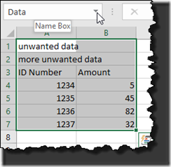
Now, I assume this data is loaded from an external file, but it doesn’t really matter, I’ll just load this from a range, as it’s just a data source. The key is that the header row is not the first row. So I defined a new range to cover the data
- Select A1:B7 –> Name Box –> Data
I can then select the name from the Name box to select my data:
I then loaded it into Power Query by creating a new query –> From Table
Determine the Header Row
This is the first job. In order to remove any rows above the header row, we need to know which row the header resides. To do that, we need to add an index column, and filter to the specific header that we’re after.
- Add Column –> Index Column –> From 0
- Filter Column1 –> only select ID Number
This results in a single row of data, and conveniently has the Index number of the ID Number row listed. In this case it’s 2.
Call up the Original Table
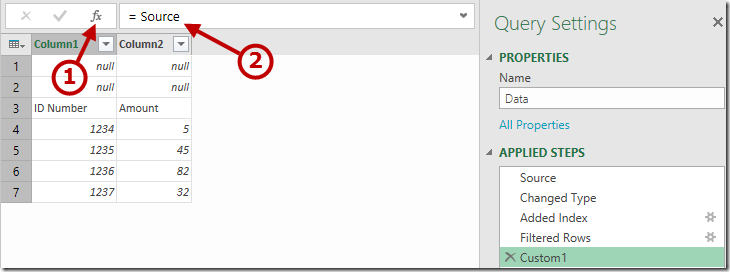
We’ll park that value for a moment, and call up the original table. To do that, we click on the fx button beside the formula bar to create a new step, then replace the formula with =Source.
Remove All Rows Up To A Specific Value
Now comes the tricky part.
We cant’ remove all rows up to a specific value immediately. We need to insert a step that removes the top 2 rows first, then modify it. So let’s do that:
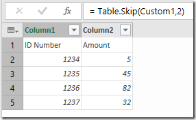
- Home –> Remove Rows –> Remove Top Rows –> 2
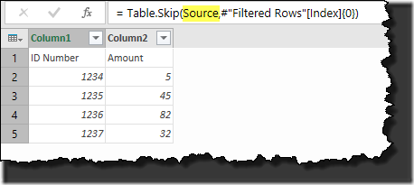
This gives us the following table and formula:
The key is to understand this formula first.
- The Table.Skip() function removes (actually skips importing) the first x rows
- Custom1 is the name of our previous step
- 2 is the number of rows
So what we really need to get is the number of rows. We can extract that from the Filtered Rows step like this:
#”Filtered Rows”[Index]{0}
Where:
- #”Filtered Rows” is the name of the step in the Applied Steps window
- [Index] is the column we want to look at in that step
- {0} indicates the first row of that step (since Power Query starts counting at 0
So let’s modify the function to:
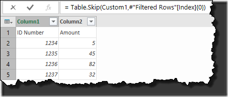
= Table.Skip(Custom1,#"Filtered Rows"[Index]{0})
As you can see, it works nicely:
In fact, we can go even better than this. Why are we referring to Custom1 at all? Doesn’t that just refer to Source anyway? Let’s also replace Custom1 with Source, and remove the Custom1 step from our query:
Cleanup
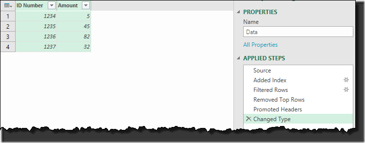
We can now promote our header rows, remove the unnecessary Changed Type step and set our data types correctly:
Testing
If you try inserting new rows at the top of the data range, then refreshing the completed query… it just works! The output table will never end up with extra rows at the top, as we’re filtering for to start at the ID Number row.
Using M
If you learn to write your own M code from scratch, you can start combining lines as well, skipping the next to explicitly filter the primary table. Bill S provided code in answer to Rudi’s question (adapted to this workbook), which is shown below:
let
Source = Excel.CurrentWorkbook(){[Name="Data"]}[Content],
AddIndex = Table.AddIndexColumn(Source, "Index", 0, 1),
Skip = Table.Skip(Source, Table.SelectRows(AddIndex, each ([Column1] = "ID Number")){0}[Index]),
PromoteHeaders = Table.PromoteHeaders(Skip)
in
PromoteHeaders
It essentially replicates the same steps as the query I built via the user interface, only he combined the Filtered Rows step into the Row Removal step. To bonus here is that the code is a bit shorter. The drawback is that it might not be quite so “de-buggable” to someone who isn’t as experienced with M.


21 thoughts on “Remove All Rows Up To A Specific Value”
This is GREAT! Ken.
I really appreciate the effort to put this together and clarify it for me. It is 100% clear now; I can see where I complicated things before and were to correct it now.
If you don't mind, I took your 'M' code example and modified it to simulate the scenario I originally faced. It was not only that the begin point was variable (ie: remove all rows above ID Number), but I also needed to remove rows below the last ID Number, or more accurately, find the heading "Purchases" which always occurs two rows below the last ID Number and remove all data from that point and below too.
So using your example, here is the resulting code for this scenario too:
let
Source = Excel.CurrentWorkbook(){[Name="Data"]}[Content],
AddIndex = Table.AddIndexColumn(Source, "Index", 0, 1),
GetIndexes = Table.SelectRows(AddIndex, each ([Column1] = "ID Number" or [Column1] = "Purchases")),
#"Kept Range of Rows" = Table.Range(AddIndex,GetIndexes[Index]{0},GetIndexes[Index]{1}-GetIndexes[Index]{0}-1),
#"Promoted Headers" = Table.PromoteHeaders(#"Kept Range of Rows"),
#"Removed Columns" = Table.RemoveColumns(#"Promoted Headers",{"3"})
in
#"Removed Columns"
TX to your posts and what I have learned from you, I am getting more confident in using 'M'. It is very powerful!!!
Cheers 🙂
Oh, BTW: A correction to the above code.
It is important to SWAP the last two lines:
#"Promoted Headers" = Table.PromoteHeaders(#"Kept Range of Rows"),
#"Removed Columns" = Table.RemoveColumns(#"Promoted Headers",{"3"})
The Remove Columns line points to a column called {"3"} which is the resulting index number after deleting the unwanted rows above. This number (which could be ANY variable number) gets promoted to a column heading and the Remove Columns step will bomb out on you as it probably will not find a column called "3" (or "8" or "24", etc)
So, SWAP the order of these two lines and ensure the first line deletes a column called "Index". Please also note to move the comma to the first of the two lines.
It should look like this:
#"Removed Columns" = Table.RemoveColumns(#"Promoted Headers",{"Index"}),
#"Promoted Headers" = Table.PromoteHeaders(#"Kept Range of Rows")
Argh.... So sorry for the stuff up!!! (My apologies!)
I should have also mentioned that the Applied Steps names must also be changed.
#"Removed Columns" = Table.RemoveColumns(#"Kept Range of Rows",{"Index"}),
#"Promoted Headers" = Table.PromoteHeaders(#"Removed Columns")
As I said above: I tend to complicate simple things!! "Sigh"
LOL! I think it's just awesome that you're working through these things! Great stuff!
Hi,
This is close to what I want but I found that columns with dates don't promote to header. I have images here:
https://twitter.com/jjrael/status/643464256587890688
I think this actually works if the excel has the first row as the header it works. I found this problem when I deleted the top rows to put the headers in the first row.
Oh, another issue is this data is actually a pivot table.
Any ideas how to make this work?
Jacob
Yes, I've see this. So here's the thing. Let's assume your column is called Column10 before you try to promote headers, and the step name (in the applied steps are is "StepName".) In a new step, you can get to that data point by referring to:
=StepName[Column1]{0}
So, given that, you can promote the rows to headers, rename the column, then edit the M code. The following should rename the column to the year from the Date column's first record:
= Table.RenameColumns(#"Promoted Headers",{{"Column10", Date.ToText(Date.From(StepName[Date]{0}),"yyyy")}})
Hope that helps,
Thanks. I will need to try that next time. My work around was to normalize the pivot table. More data coming in but I don't have dates as headers. BTW, my dates will change each month. Will your solution work for that case? I didn't know if "yyyy" was a formatting string or if I needed to replace that with the actual date.
It should work, yes. The "yyyy" is a formatting string.
Thanks for the clear and straightforward instruction, Ken. I was able to update my query to accommodate additional header rows in 15 minutes start to finish.
An alternative solution for:
Skip = Table.Skip(Source, Table.SelectRows(AddIndex, each ([Column1] = "ID Number")){0}[Index]),
Would be:
Skip = Table.Skip(Source,Table.RowCount(Table.FirstN(Source,each [Column1] "ID Number"))),
This solution doesn't require an index column.
The "not equal" (less than, greater than) got lost when I posted my comment.
My code should read:
Skip = Table.Skip(Source,Table.RowCount(Table.FirstN(Source,each [Column1] NotEqual "ID Number"))),
Even simpler:
Skip = Table.Skip(Source,[Column1] NotEqual "ID Number")
Terrific Marcel. NB had to add the 'each' keyword to your last note, and for the life of me I can't work out how the literal 'NotEqual' works - it certainly crashes enthusiastically on my machine (Excel 2016). This works for me:
Skip = Table.Skip(Source, each [Column1] "DooWop")
Aha!!! I see why you wrote 'NotEqual'!!! Because "" don't appear on the post! Let's try putting quotes around em and see what happens .....
ok, for dummies like me, make sure you use the normal arithmetic operators for NotEquals. While I had originally tried the arithmetic operators myself, the missing 'each' was also producing an error, which confused me. Happy days folks.
Nice one ! Also like Marcel's approach.
I found one another solution to get the correct number of row(s) to skip:
RowsToRemove = List.PositionOf( Source[Column1], "ID Number")
It doesn't require any index column / filter !
Pingback: Power Query (M)agic: Dynamically remove leading rows AND columns - PowerPivotPro
Ken - thanks for the post - managed to follow and remove all the unwanted data
Tristan - even better solution - switched my code to yours now
Hi Ken, this is an amazing thing to have in the toolkit. Thanks so much for putting this post together and explaining it in such a graceful way.
Hi Ken, Ditto on previous comments, this was great instruction. I applied the same logic to remove an unknown number of trailing rows. Thanks!
Hello,
I have a situation where I need to keep all the rows except the maximum. I'm parsing a PDF file with different number of tables each time. Client can't/won't change from PDF format to something useful like csv.
Due to layout of the PDF, I have to treat page 1 and the final page differently from the middle pages.
For the middle section, I need to keep all the rows except for those on the final page of the PDF. I'm thinking I might be able to re-work the logic from this post, but would appreciate some guidance.
Thank you,
Matthew