Earlier this week I received an email asking for help with a Power Pivot model.  The issue was that the individual had built a model, and wanted to add slicers for value fields.  In other words, they’d built the DAX required to generate their output, and wanted to use those values in their slicers.  Which you can’t do.  Except maybe you can…  🙂

My approach to solve this issue is to use Power Query to load my tables.  This gives me the ability to re-shape my data and load it into the data model the way I need it.  I’m not saying this is the only way, by any means, but it’s an approach that I find works for me.  Here’s how I looked at it in Excel 2013.  (For Excel 2010 users, you have to run your queries through the worksheet and into Power Pivot as a linked table.)

Background

The scenario we’re looking at is a door manufacturer.  They have a few different models of doors, each of which uses different materials in their production.  The question that we want to solve is “how many unique materials are used in the construction of each door?”  And secondarily, we then want to be able to filter the list by the number of materials used.

The first question is a classic Power Pivot question.  And the setup is basically as follows:

• Download the sample file here
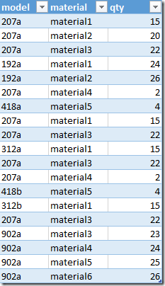
• Use Power Query to pull the MaterialsList table (shown below) into Power Pivot.

• Create a PivotTable with models on rows and material on columns
• Create a DAX measure to return the distinct count of materials:
  • DistinctMaterials:=  DISTINCTCOUNT(MaterialsList[material])
• Add a little conditional formatting to the PivotTable if you want it to look like this:

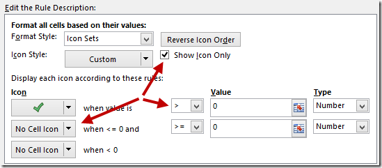
The secret to the formatting is to select the values and set up an icon set.  Modify it to ensure that it is set up as follows:

Great stuff, we’ve got a nice looking Pivot, and you can see that our grand total on the right side is showing the correct count of materials used in fabricating each door.

Creating Slicers For Value Fields

Now, click in the middle of your Pivot, and choose to insert a slicer.  We want to slice by the DistinctMaterials measure that we created… except.. it's not available.  Grr…

Okay, it’s not surprising, but it is frustrating.  I’ve wanted this ability a lot, but it’s just not there.  Let’s see if we can use Power Query to help us with this issue.

Creating Queries via the Editor

We already have a great query that has all of our data, so it would be great if we could just build a query off of that.  We obviously need the original still, as the model needs that data to feed our pivot, but can we base a query off a query?  Sure we can!

• In the Workbook Queries pane, right click the existing “MaterialsList” query and choose Edit.
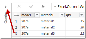
• You’ll be taken into the Power Query editor, and on the right side you’ll see this little collapsed “Queries” window trying to hide from you:

• When you expand that arrow, you’ll see your existing query there!
• Right click your MaterialsList query and choose “Reference”.

You’ve now got a new query that is referring to your original.  Awesome.  This will let us preserve our existing table in the Power Pivot data model, but reshape this table into the format that we need.

Building the Query we need

Let’s modify this puppy and get it into the format that will serve us.  First thing, we need to make sure it’s got a decent name…

• On the right side, rename it to MaterialsCount

Now we need to narrow this down to a list of unique material/model combinations, then count them:

• Go to Add Column –> Add Custom Column
• Leave the default name of “Custom” and use the following formula:  [model]&[material]
• Sort the model column in ascending order
• Sort the material column in ascending order

We’ve not got a nicely ordered list, but there’s a few duplicates in it.

Those won’t help, so let’s get rid of them:

• Select the “Custom” column
• Go to Home –> Remove Duplicates

Now, let’s get that Distinct Count we’re looking for:

• Select the “model” column
• Go to Transform –> Group By
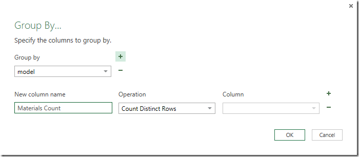
• Set up the Group By window to count distinct rows as follows:

Very cool!  We’ve now got a nice count of the number of distinct materials that are used in the production of each door.

The final step we need to do in Power Query is load this to the data model, so let’s do that now:

• File –> Close & Load To…
• Only create the connection and load it to the Data Model

Linking Things in Power Pivot

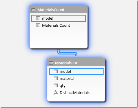
We now need to head into Power Pivot to link this new table into the Data Model structure.  Jump into the Manage window, and set up the relationships between the model fields of both tables:

And that’s really all we need to do here.  Let’s jump back out of Power Pivot.

Add Slicers for Value Fields

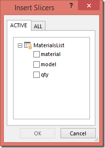
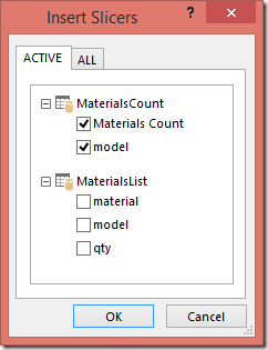
Let’s try this again now. Click in the middle of your Pivot and choose to insert a slicer.  We’ve certainly got more options than last time!  Choose both fields from the “MaterialsCount” table:

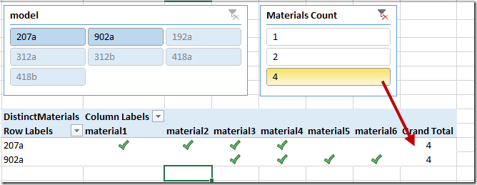
And look at that… we can now slice by the total number materials in each product!