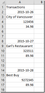
For the first post of the new year, I thought I’d tackle an interesting problem; how to Transpose Stacked Tables in Power Query. What’s do I mean by Stacked Tables? It’s when your data looks like this:
Notice that we’ve got 3 tables stacked on top of each other with gaps. The question is, how do we deal with this?
There’s actually a variety of different ways we could accomplish this, but I want to show a neat trick that allows us to refer to data on the next row(s) in Power Query this time. We may revisit this in future with some other techniques as well, but for now… I think you’ll find this interesting.
Sample File
If you’d like to play along, click here to download the sample file, with a mock-up of a fictional Visa statement.
Getting Started
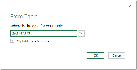
The first thing we need to do is pull the data into Power Query, so let’s go to Power Query –> From Table, and set the range to pull in all the data from A1:A17:
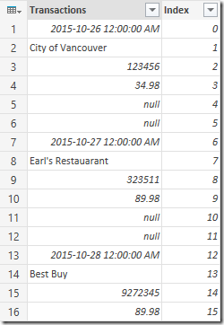
We end up with the table in the Power Query window, and we’re now going to add an Index column to it; something you’re going to see can be very useful! To do this, go to Add Column –> Add Index Column (you can start from 0 or 1, your preference. I’m just going to go with 0):
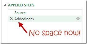
Now, for simplicity, I am going to make an unnecessary change to start with. What I’m going to do is – in the “Applied Steps” section, I’m going to right click the “Added Index” line, and choose Rename, then rename this step to “AddedIndex” with no space:
Transpose Stacked Tables - The Tricky Part
Go to Add Column –> Add Custom Column. In the window that pops up:
- Name the column “Location”
- In the formula area, enter: AddedIndex{[Index]+1}[Transactions]
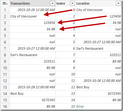
And the result:
Wow… how cool is that? We’ve referred to the value on the next row! But how? The secret is in the syntax. It basically works like this:
Name of previous step{[Index] + 1}[Name of Column to Return]
Watch all those brackets carefully too. The curly ones go around the index row you want to return (the index number of the current row plus 1), and the square brackets around the name of the column you want.
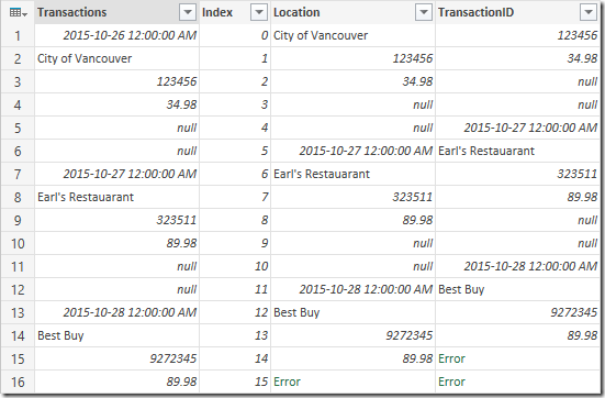
Now, let’s do the next row. Add a new column again:
- Name the column “TransactionID”
- In the formula area, enter: #”Added Custom”{[Index]+2}[Transactions]
Okay, so what’s with that? Why the # and quotes around the previous step this time? The answer is that, in order to read the column name with the space, we need to wrap the column’s name in quotes and preface it with the # mark. This tells Power Query to interpret everything between the quotes as a literal (or literally the same as what we wrote.) As you can see, it works nicely:
Just to circle back on the unnecessary step I mentioned before, it was renaming the “Added Index” step. Doing that saved me having the type #”Added Index”. Personally I can’t stand all the #”” in my code, so I tend to modify my steps to drop the spaces. It looks cleaner to me when I’m reading the M code.
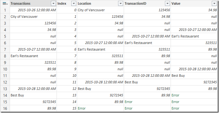
At any rate, let’s do the last piece we need too. Add another column:
- Name the column “Value”
- In the formula area, enter: #”Added Custom1”{[Index]+3}[Transactions]
Beautiful… I’ve got each row of data transposed into the table the way I need it, but I’ve still got a bunch of garbage rows…
Taking Out The Trash
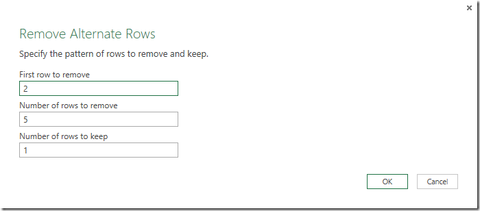
As it stands, we really only need the rows that start with the dates. Again, we have multiple options for this, but I see a pattern I can exploit. I need to:
- Keep 1 row
- Remove 5 rows
- Repeat
How do we do that easily? Go to the Home Tab –> Remove Rows and choose Remove Alternate Rows!
And finally we can get rid of the Index column, set our Data Types, and we’re all set:
And there you have it. Just one of a few ways to Transpose Stacked Tables using Power Query.



12 thoughts on “Transpose Stacked Tables”
Hehe...what I see? :-))
Greetings
A technique I learned from an email that landed in my inbox. 😉
Ok... no offence 🙂
I presented this technigue a month ago in this video:
https://www.youtube.com/watch?v=iH--rbWgTUY
Back to this topic... This is possible also by clicking only
Code below can do that.
let
Source = Excel.CurrentWorkbook(){[Name="tblTransactions"]}[Content],
Filter1 = Table.SelectRows(Source, each ([Transactions]<>null)),
AddedIndex = Table.AddIndexColumn(Filter1, "Indeks", 0, 1),
AddMod = Table.AddColumn(AddedIndex, "Wstawiono modulo", each Number.Mod([Indeks], 4), type number),
ChType = Table.TransformColumnTypes(AddMod,{{"Wstawiono modulo", type text}}),
Pivot1 = Table.Pivot(ChType, List.Distinct(ChType[Wstawiono modulo]), "Wstawiono modulo", "Transactions"),
FillUp1 = Table.FillUp(Pivot1,{"1", "2", "3"}),
Filter2 = Table.SelectRows(FillUp1, each ([0]<>null)),
RemCol = Table.RemoveColumns(Filter2,{"Indeks"}),
RenCol = Table.RenameColumns(RemCol,{{"0", "Date"}, {"1", "Name"}, {"2", "Id"}, {"3", "Value"}}),
ToDate = Table.TransformColumns(RenCol,{{"Date", DateTime.Date}}),
ChType2 = Table.TransformColumnTypes(ToDate,{{"Id", Int64.Type}, {"Value", type number}})
in
ChType2
oops.... WordPress ate some parts of code 🙁 so... here is a link to the file (clicking solution) on my google drive
https://drive.google.com/file/d/0B6UlMk8OzUrxSkZjYlJ2SUx6VVU/view?usp=sharing
Hi Bill,
Thanks for posting. I've modified the code above to insert the eaten chunks.
I agree that the method I posted isn't the easiest, but I do like the ability to refer to that next row. Not sure how often I'll need it, but one day, when there isn't another option, I'm sure it will come in useful.
Looking at the code you posted, I wonder if it might be time to do a post on Pivot. I know Chris has already done one, and your code does it, but I don't think I have yet. 🙂
I'd rather look at arrays:
Sub M_snb()sn = [a2:A55]
ReDim sp(UBound(sn) \ 6, 3)
For j = 1 To UBound(sn) Step 6
For jj = 0 To 3
sp(j \ 6, jj) = sn(j + jj, 1)
Next
Next
End Sub
Kevin Lehrbass also shared a technique using formulas. http://youtu.be/iVtgwJmp7Fg
Lots of ways to do this, for sure. 🙂
It was good practice! I should try solving it using VBA. I'm really rusty.
hehe... accidentally, I have read this post on MrExcel Message Board and now i understand "from an email that landed in my inbox" 🙂
http://www.mrexcel.com/forum/power-bi/822788-power-query-filter-columns-condition.html#post4018579
By the way, the use of Table.Range and Table.Transpose would probably be better in this case (but this is not only "by clicking" way)
@ Ken your code assumes that each stack has the same no of rows
The below code is more generic
Assuming no header row in the Data for the table called D
let
Source = Excel.CurrentWorkbook(){[Name="D"]}[Content],
mBlk = Table.FromRecords({[Column1= null]}),
mAppendQ = Table.Combine({Source,mBlk}),
mAddIndex = Table.AddIndexColumn(mAppendQ, "Index", 0, 1),
mAddCustom = Table.AddColumn(mAddIndex, "Custom", each if [Column1] = null then [Index] else null),
mFillUp = Table.FillUp(mAddCustom,{"Custom"}),
mRemCols = Table.RemoveColumns(mFillUp,{"Index"}),
mGrpRows = Table.Group(mRemCols, {"Custom"}, {{"Table", each Table.Transpose(Table.SelectColumns(_,{"Column1"})), type table}}),
mNoOfCols = Table.Max(Table.AddColumn(mGrpRows, "ColCount", each Table.ColumnCount([Table])),"ColCount"),
mCols = {1..mNoOfCols[ColCount]-1},
mCovToTbl = Table.FromList(mCols,Splitter.SplitByNothing()),
mChgTyp = Table.TransformColumnTypes(mCovToTbl,{{"Column1", type text}}),
mAddColNms = Table.AddColumn(mChgTyp, "Custom", each "Column"&[Column1]),
mRemOthCols = Table.SelectColumns(mAddColNms,{"Custom"}),
mTblToLst = Table.ToList(mRemOthCols),
mRemCols1 = Table.RemoveColumns(mGrpRows,{"Custom"}),
mExpandTbl = Table.ExpandTableColumn(mRemCols1, "Table", mTblToLst, mTblToLst),
mRemDups = Table.Distinct(mExpandTbl)
in
mRemDups
Cool stuff, Sam. Thanks for sharing!
Pingback: Re-arrange, Rotate, Transpose, Twist, Cascade the data! | My Spreadsheet Lab