My last few posts have been relatively technical, so this time I figured I’d look at something practical.  I can’t believe it’s been almost a year since I blogged about un-pivoting data in Power Query, so it’s about time we looked at that again… but this time with a twist.  This time we’ll look at un-pivoting with subcategories in Power Query.

Background

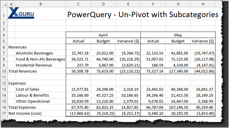
The data we’re going to start with looks like a typical financial report.  Whether a restaurant or a shoe store, in the manager’s office you’re liable to come up with a report that looks something along the lines of this:

Now for the challenge… someone decides they need an alternate view of this data.  So how do you quickly un-pivot this into a format that you can use for other things?

If you want to follow along, you can download the file from my OneDrive.

Issue 1 – Getting the Data into Power Query

The first issue we come across is that, while Power Query can consume data from inside an Excel file, it MUST be formatted as a table.  But this hardly looks like it’s conducive to a table format with all those blank rows and such.  But what the heck… let’s apply a table to it anyway, and see what happens.

• Click anywhere
• Choose Power Query –> From Table
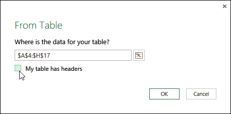
• Adjust the range to cover all of the data (A4:H17)
• Uncheck the box that indicates your table has headers

When you’re done, the box should look as follows:

And when you say OK, you should be taken into Power Query.

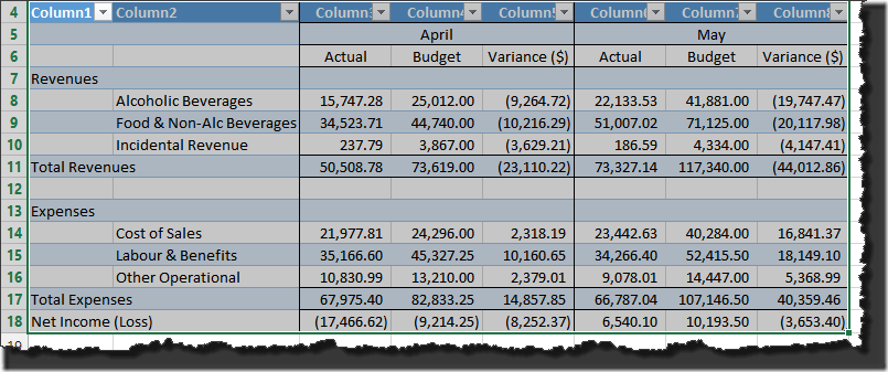
If you take a quick peek back at Excel, you can see that the table has indeed been applied, and that there are generic column headers above each column:

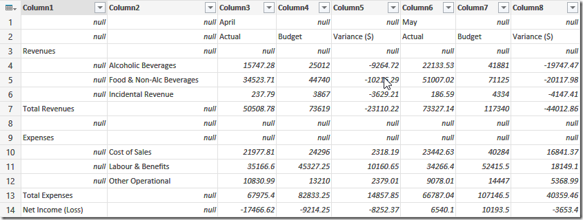
This is also reflected in Power Query:

Data Cleanup

Before we get into the trick of how to deal with subcategory columns, let’s clean up some of the garbage here.  Ideally what we’d like to get here is a nice pure table that we can easily un-pivot, just like we did in the prior article.

Cleanup Step 1:

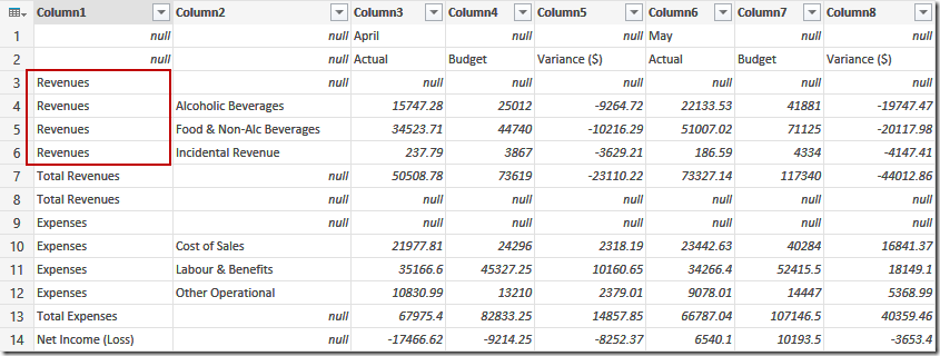
Looking at the first column, we’ve got a bunch of null values in there, as well as some section headers.  What we really need is those section headers repeated on the lines below them.  So let’s make that happen.

• Select Column1
• Go to Transform –> Fill –> Down

You’ll see that the section headers are filled into any of the null areas. As soon as they encounter data however, they stop. (I’ve drawn a box around the Revenue lines below – notice how they fill until they reach Total Revenues, which then fill until they reach Expenses, and so on.)

Cleanup Step 2:

Now, we don’t really need any of the rows that are showing null values in Column3 through Column 8.  Let’s filter Column3 to remove those.  Click the drop down on Column3 and uncheck (null).  The result looks like this:

So… why didn’t I filter the null values out of Column2?  After all, there are blank data rows, and with a PivotTable we can recreate the subtotals…  The answer is that I’m not ready to lose the first two rows yet.  I need those in order to un-pivot my data. 😉

Issue 2 – Un-Pivoting the Data

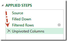
If things were lined up perfectly, we could just select Column3 through Column 8 and un-pivot it now.  Unfortunately, if we do we’ll get some really wonky results.  (Go ahead and try it if you like. Remember to click the x to the left of the “Unpivoted Columns” step once you confirm you’ve made a disaster of it!)

Preparing to Un-Pivot

Okay, so what do we need to do… well, the first thing we need to do is fill the first row (containing April and May) across the columns.  Here’s the rub though… there is no Fill—>Across feature.  So how do we do it?

Transposing the Table

To an accountant, transposition is an evil word that means you made a mistake and flipped two digits around.  It’s nasty and something we never look forward to.  But to Power Query it’s simply awesome.  Check this out…

• Go to Transform—>Transpose

This instantly flips the columns to rows and rows to columns!

And would you look at that… April and May are in Column1 and below them… null values!  We know what to do with those now!

• Select Column1
• Go to Transform –> Fill –> Down

Is this enough though?  Nope, sorry.  You might be tempted to “un-transform” and then un-pivot it, but you’d still end up with garbage.  We still need to do a bit more.

Concatenating the Category and Subcategory

This is the trick to un-pivoting with subcategories: you need to concatenate them first, then un-pivot, then split them up.  So let’s get to it.  Using the tip from Merging Columns with Power Query, let’s join up Column1 and Column2.

• Select Column1
• Hold down CTRL or SHFT and select Column2
• Click Transform –> Merge Columns
• Choose the Colon for the separator (or whichever you prefer)

Note:  If you don’t have the Merge Columns feature, you’re using an old version of Power Query. Either download the latest version, or you’ll need to manually join the columns by:

• Adding a new column
• Using the formula =[Column1]&”:”&[Column2]
• Delete Column1 and Column2
• Move the new column to the first position

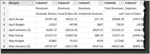
Once you’ve got it done, the output should look as follows:

Un-transposing the Table

Awesome… we’ve got concatenated headers now.  We just need to flip the table back right side up and we’re almost ready to un-pivot it:

• Go to Transform –> Transpose

Final Preparations

The very last thing we need to do before we un-pivot our table is provide some decent headers.  This will ensure that the data will make sense when it is un-pivoted.  To that end:

• Go to Transform –> Use First Row as Headers
• Rename the first column to “Class”
• Rename the second column to “Category”
• Filter “Category” to remove the null values

Our table now looks nice and clean:

And we’re ready!

Un-Pivot It!

We now follow the steps of a regular un-pivot operation, with only a minor extra step:

• Select the Class column
• Hold down CTRL or SHFT
• Select the Category column
• Go to Transform –> Unpivot Columns –> Unpivot Other Columns
• Rename the “Value” column to “Amount”

And now the extra step:

• Select the “Attribute” column
• Go to Transform –> Split Column –> By Delimiter –> Colon
• Rename the Attribute.1 column to “Month”
• Rename the Attribute.2 column to “Measure”

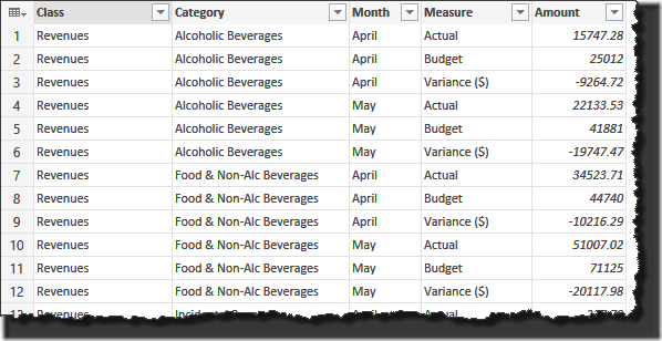
The results:

That’s pretty much it.  The last thing I’d do is change the Query name from Table1 to something more intelligible… maybe Data or something… then load it to the worksheet.

From a Static Report to a Data Source

Now that we’ve got our report reformatted into a data source, we can click anywhere in the table and pivot it to our heart’s content!

A Quick Recap

To be fair, this post has been pretty long, but only because I included a LOT of pictures and detailed instructions.  Once you’ve got the process nailed down, it doesn’t take all that long at all.  Remember, the big key to this is:

• Suck your report into a table (without headers)
• Fill any rows you can
• Transpose the data
• Concatenate your category and subcategory fields together
• Un-transpose it
• Un-pivot it
• Split the category and subcategory back into their pieces

Enjoy!  🙂