The comments of my last post collected a tip that I thought it was worth exploring on pulling Excel named ranges into Power Query.
I made the claim that Excel MUST have the data in an official Excel table. As LoganEatsWorld pointed out, that’s actually not true any more. If you’d like to give this a go, you can download this workbook to follow along.
What’s in the file?
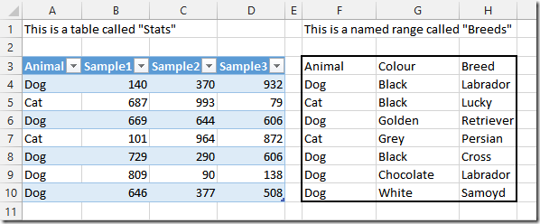
The file is very basic. It simply contains one table, and one named range of data:
The table is highlighted in the blue table style, and bears the name “Stats”. The named range is surrounded by the black outline, and is called “Breeds”.
Connecting to Excel Data:
The reason I never found this is that my method was always to go to the Power Query tab and click –> From Table. That will work great to get the data out of a table, but it won’t work for the named range. So let’s try this a different way…
- Go to Power Query –> From Other Sources –> Blank Query
- Click in the formula bar and type the following:
= Excel.CurrentWorkbook()
(Yes, it’s case sensitive… I’m starting to reconcile myself to the fact that it’s Power Query so I’m just going to have to get over it.)
What ends up happening is a bit of magic:
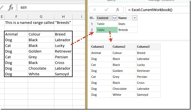
Interesting… we have two tables listed! The first is our official table, the second is our named range. Cool!
Let’s click in the blank space to the right of the green “Table” text in the Breeds row:
The preview pops up and, sure enough, that’s our named range data:
Working With The Data
All right, let’s click the green Table text and break open that named range:
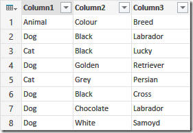
One notable difference here (in fact really the only one), is that Power Query doesn’t automatically recognize the header row. This is due to the fact that an Excel table actually has a named header row to promote, where a named range does not. No big deal though, as we can easily deal with that:
- Go to Transform –> Use First Row As Headers
At this point, we could save the table to the worksheet or data model, as we need.
Observations
So this is cool. It’s awesome that we can get to named ranges, as I have a LOT of workbooks that use these, and there are occasions where I don’t want to convert them to official Excel tables. Despite the fact that we can, however, you pretty much need a secret decoder ring to find it, and that’s not so good.
It would sure be nice if there was a more discoverable way to pull in a named range… but where?
Suggested Accessibility Option 1
When I look at Power Query’s “Get External Data” function, it seems logical to me that it should end up somewhere in that area. Looking at the group:
I kind of like the ability that comes with the “From Table” feature which works from the table you’re in (if you are), and lets you create a table if you’re not inside a table when you click that button. But I wonder if it would be better served as a SplitButton/menu/submenu structure that offered the following options:
- From Table
- Current Table
- Other Table
- List of other tables in the workbook
- Named Range
- List of named ranges in the workbook
- Create New Table
- Create New Named Range
Actually, there is another change I would make to that group, and that’s to move the “From Blank Query” out of the “From Other Sources”, and give it it’s own button. (I create a LOT of queries from scratch now, and it’s just extra clicks in my way to do so.)
Suggested Accessibility Option 2
I’m not sure this is so much of an alternate as something additional I’d like to see, actually. An “additional sources” button on the Home tab would be awesome. If that had the ability to pull up all the existing tables or named ranges in the workbook, and add them to the Power Query script as a “Source2=…”
I think the implications of this would be two fold:
- It would allow you to add a data source after creating a blank query, and/or
- It would allow you to add additional data sources into the same query.
The latter is certainly something I do semi frequently, as I don’t want to have multiple Power Queries created that are then merged together. I’ll add both sources manually in the same query then merge them.
At any rate, just some thoughts. If you have any on the subject please feel free to leave them in the comments. 🙂


20 thoughts on “Pulling Excel Named Ranges into Power Query”
Some further information and observations from Chris Webb can also be found here: http://cwebbbi.wordpress.com/2014/07/22/working-with-excel-named-ranges-in-power-query/
Ken,
I will typically use the "From File" drop down menu and then select "From Excel" and then select the workbook that I am currently working in. This allows me to consume excel data in PQ from a worksheet, table, or a named range.
Thanks for the great tips.
Hi Dave,
That's an interesting approach, but I'd be pretty cautious in using it. While it gives you a lot of flexibility to pull in more ranges, it also hard codes the external path to the workbook in your M code. If you made a copy of the workbook I think you'll find that the M still points to the original workbook. That could lead you to unexpected results, not to mention queries that break if you send the workbook to someone who doesn't have access to the original file's location.
I keep hoping that they'll implement a "CurrentWorkbook.Path" object in the M code. That would be SUPER useful, as you could then nest that in to avoid this kind of challenge.
Ken,
In response to your comment about adding a separate button for "From Blank Query", what I did was add the "From Blank Query" button to the Quick Access Toolbar. (Although I agree with you that having it as a separate button in the ribbon for the Power Query tab would be nice.)
Your suggestions for the "from current workbook" selections is right on the money.
Pingback: Excel Roundup 20141006 « Contextures Blog
Hmm... yes, pinning it to the QAT would work. I try to keep my QAT pretty clean, personally. Not sure why, just personal preference, I guess.
You could also customize the ribbon to add it to the Power Query ribbon too. You have to add a new group, and then add the Blank Query button. Interestingly it always sorts that group to first position on my system, no matter where you move it to...
Ken,
Excellent tip! You improved my table creation process.
I have two PQ's that create separate tables/named ranges ('import1' and 'import2')
Old method
1) the tables are merged into one master table. Unfortunately this 'reruns' the two PQ's to create the merged master table. Takes a bit of time.
New method
2) Now I use Table.Combine to combine the previously created tables/named ranges. Quick since it uses the already created tables/named ranges.
Sample code:
let
Source = Excel.CurrentWorkbook(),
_import1 = Source{[Name="_import1"]}[Content],
#"Appended Query" = Table.Combine({_import1, Source{[Name="_import2"]}[Content]})
in
#"Appended Query"
Hey Doug,
Do be a bit careful there. I would prefer to set up two separate queries, one for _import1 and one for _import2, and set both as connection only. From there, combine them in one query:
let
Source = Table.Combine({_import1,_import2})
in
Source
The reason for this is that you are guaranteed to avoid the formula firewall. It may not bite you today, but getting your stuff into a staged format will protect you in the future.
Hi. I'm new to Power Query. I'm currently working with loads of Excel/CSV files. Each file has a varying number of columns in varying order. Column names are consistent in all the files though. For example, in file 1, Age is in Column 3 and Name is in Column 4, while in file 2, it's the other way around. When I import the files through PQ using the From Folder option, the columns are combined in such a way that Column 3 will have both Age and Name in it. This is true with both Excel and CSV files.
Is there a way to direct PQ to extract columns based on column names instead of order? Please help.
Hi Rache,
Yes, there is a way, it's just a bit complicated today. What version of Excel are you using?
The reason I'm asking is that we're expecting to see a new version of Power Query released for Excel 2010/2013 within the next couple of weeks that includes the new Combine Binaries experience that I blogged about here: https://excelguru.ca/2016/12/22/combine-excel-files. This will actually make the job really easy, as you'll be able to promote the column names BEFORE the files are consolidated. This means that you won't have issues with the columns being mis-combined.
We can do this without the new update, but it will take a custom function in order to pre-process the data. This is something that we cover in Chapter 21 of M is for Data Monkey (http://xlguru.ca/monkey), and you can also find some examples of building custom functions on the blog as well.
Hi,
If I want to bring range from other workbook. The range is a offset formula. I can't bring it, there is no option.
Help 😛
Hey Igor,
I don't believe you'll be able to pull a dynamic named range from another workbook. As the Excel workbook is closed, it won't be able to evaluate the array formula, so you're dead in the water.
A better method may be to pull in the entire worksheet. If you can set up some formulas in the workbook that evaluate the first row/last row and first column/last column of the dynamic range, those will get saved in the workbook. Then you could read those to know how to get rid of the remaining data.
Hi Ken.
I am a big fan of yours and I have asked my analyst to take a PD course you are teaching on July 4/5 on this. She is super excited.
I have a question for you. I want to pull multiple named ranges (instead of tables) on multiple tabs into one Query. The challenge I have is the promoting headers. As soon as I promoted the headers (for example 100 columns of dates), I have trouble loading the Query. It works fine with tables with headers and alternatively I can manually name the headers in query editor but it’s 100 of headers. Is there a way to get the headers from named ranges in multiple tabs automatically?
Hi Michael, thanks for this, and am looking forward to the course!
With your exact question, I'd honestly need to see your query to get an idea of how to slice it up.
I'm combining this with named ranges linked to spill cells to get scalable date tables (for example)
Thank you!!
Thanks Ken and others for the above insights. I am a complete rookie at PQ and have never posted to any forum in my life so treat the below with some caution.
This is how I have been accessing Named Ranges, avoiding the often-mentioned solutions of bridging queries and/or functions. Here is select a file to load and then filter by two different columns where all variables are set in Named Ranges in the Spreadsheet.
It works fine for me but I am not sure how long my (beginner's) luck will hold 😉
let
/* USER Variables:
File = the name of the input file parameter stored in the Named Range "p.File"
FilterH = the value of the filter parameter for House Type stored in the Named Range "p.House"
FilterS = the value of the filter parameter for Service Type stored in the Named Range "p.Service"
*/
File = Excel.CurrentWorkbook(){[Name="p.File"]}[Content][Column1]{0},
FilterH = Excel.CurrentWorkbook(){[Name="p.House"]}[Content][Column1]{0},
FilterS = Excel.CurrentWorkbook(){[Name="p.Service"]}[Content][Column1]{0},
Source = Excel.Workbook(File.Contents(File), null, true),
Sheet1_Sheet = Source{[Item="Sheet1",Kind="Sheet"]}[Data],
#"Promoted Headers" = Table.PromoteHeaders(Sheet1_Sheet, [PromoteAllScalars=true]),
#"Changed Type" = Table.TransformColumnTypes(#"Promoted Headers",{{"LocationID", type text}, {"House Type", type text}, {"Service", type text}}),
#"Filtered Rows" = Table.SelectRows(#"Changed Type", each ([House Type] = FilterH) and ([Service] = FilterS))
in
#"Filtered Rows"
Hi Peter, I believe that - with all your variables declared as separate steps up front - you should be good. I'd still prefer to create a separate query for each data source, but that's just my preference. 🙂
Hi Ken,
Thank you for all the very useful information you publish.
My question is can PQ import a value from a named range where the value is stored directly in the named range and not on a worksheet.
I am trying to do it this way to avoid the need to have a cell value on a (additional) worksheet which creates clutter and can be accidently deleted etc.
I populate the named range using the following vba code.
ActiveWorkbook.Names("strPath").RefersToR1C1 = "xxx"
Thanks Geoff
Hi Geoff,
Unfortunately no. PQ restricts to only look at named ranges that point to cell ranges. 🙁