My recent post on showing the Top X with Ties inspired a discussion on ranking methods.  Where I was looking to rank using what I now know as a standard competition rank, Daniil chose to use a dense ranking method instead.  Oddly, as an accountant, I've never really been exposed to how many different ways there are to rank things - and I'd certainly never heard the terms skip and dense before. (At least not tied to ranking!)

Naturally, after a few emails with Daniil and a bit of a read over at Wikipedia on 6 different common ranking methods, I had to see if I could reproduce them in Power Query.

What are the 6 different ranking methods?

Let's look at a visual example first.   These were all created in Excel using standard formulae:

The first thing I had to do was figure out what each ranking method actually does.  So here's a quick summary according to Wikipedia's article on the subject:

• Ordinal Ranking - This ranking method uses sequential number for each row of data, without concern for ties
• Standard Competition Ranking - Also know as a form of a Skip ranking, this method gives ties the same rank, but the following value(s) are skipped.  In this case, our values go 1,2,3,4,4, 6.  (5 is skipped as the 5th item is tied with the 4th)
• Modified Competition Ranking - This is similar to the Standard Competition ranking method, but the skipped values come before the ties.  In this case, we would get 1,2,3, 5, 5, 6.  (As 4 and 5 are tied, they both get ranked at the lower rank.)
• Dense Rank - In this ranking method, ties are given the same value, but the next value is not skipped.  In this case we have 1, 2, 3, 4, 4, 5.
• Fractional Rank - Now this one is just weird to me, and I'd love to know if anyone has actually used this ranking method in the real world.  In this algorithm, ties are ranked as the mean of the tied ordinal rank.  Very strange to me, but it won't stop me from building it!

So know that we know what they all are, let's build them in Power Query so that we can perform them in both Power BI and Excel.

Groundwork for demonstrating the ranking methods

If you download the sample workbook, you'll see that it has the full table shown above.  To make this easy, I set up a staging table called SalesData as via the following steps:

• Select a cell in the Excel table --> Data --> From Table/Range
• Select the Item and Sales columns --> right click --> Remove Other Columns
• Load it as a connection only

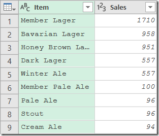
This gave me a simple table with only the product names and values as shown here:

As you can see, the values column has already been sorted in descending order, something that is key to ranking our ties.

One thing I should just mention now is that - for every ranking method - we will actually start every new query by:

• Referencing the SalesData query
• Renaming the new query to represent the ranking method being demonstrated

That means that I'm just going to give the steps each time based on the view above, since that's what we should get from the referencing step.

Ranking Method 1: Ordinal Rank

This ranking method is super easy to create:

• Sort the Sales column in descending order
• Sort the Item column in ascending order (to rank ties alphabetically)
• Go to Add Column --> Index Column --> From 1
• Rename the Index column to Rank
• Reorder the columns if desired

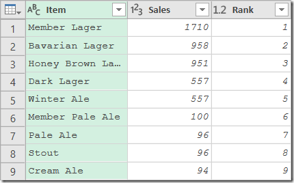
Yes, that's it.  It simply adds a row number to the way you sorted your data, as shown  here:

Ranking Method 2: Standard Competition Rank

This ranking method involves using a little grouping to get the values correct:

• Sort the Sales column in descending order
• Add an Index column from 1
• Go to Transform --> Group
  • Group by the Sales column
  • Create the following columns:
    • Rank which uses the Min operation on the Index column
    • Data which uses the All Rows operation
• Expand the Item column
• Reorder the columns if desired

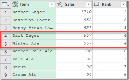
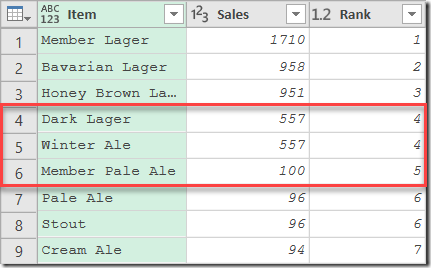
The result correctly shows that the Dark Lager and Winter Ale - 4th and 5th in the list, but tied at 557, each earn a rank of 4, and the Member Pale Ale (6th in the list) comes in with a rank of 6.  There is no item ranked 5th, since their rank was improved to be in a 4th place tie.

Ranking Method 3: Modified Competition Rank

To create ranking following the Modified Competition ranking method, we need to:

• Sort the Sales column in descending order
• Add an Index column from 1
• Go to Transform --> Group
  • Group by the Sales column
  • Create the following columns:
    • Rank which uses the Max operation on the Index column
    • Data which uses the All Rows operation
• Expand the Item column
• Reorder the columns if desired

The only real difference between this ranking method and the standard competition rank is that we create the Rank column using the Max of the Index column instead of the Min used in the previous method.

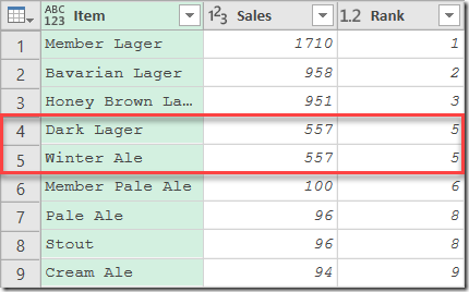
The result correctly shows that the Dark Lager and Winter Ale - 4th and 5th in the list, but tied at 557, now earn a rank of 5 (not 4 like the standard rank).  There is no item ranked 4th, since their rank was dropped to reflect a 5th place tie.

Ranking Method 4: Dense Rank

The dense ranking method requires a change to the order of the steps from what we did in the standard competition ranking method.  Namely the Group By command must come before the addition of the Index column:

• Sort the Sales column in descending order
• Go to Transform --> Group
  • Group by the Sales column
  • Create the following columns:
    • Data which uses the All Rows operation
• Add an Index column from 1
• Expand the Item column
• Reorder the columns if desired

This method will yield the results found here:

The result correctly shows that the Dark Lager and Winter Ale - 4th and 5th in the list, but tied at 557, ranked in 4th place - just the same as the Standard Competition rank.  But where it differs can be seen in the ranking of the Member Pale Ale.  6th in the list, it is ranked 5th, as there are no gaps left after the ties.

Ranking Method 5: Fractional Rank

As I mentioned at the outset, I find this to be one of the strangest methods of ranking.  Like the others though, it's actually really easy to create when you know how. (And certainly more straight forward than using an Excel formula to calculate it!)

• Sort the Sales column in descending order
• Add an Index column from 1
• Go to Transform --> Group
  • Group by the Sales column
  • Create the following columns:
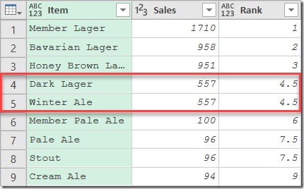
    • Rank which uses the Average operation on the Index column
    • Data which uses the All Rows operation
• Expand the Item column
• Reorder the columns if desired

One thing I will say… it's certainly makes it obvious that there are other ties in the table.  Maybe that's the point of it?

Final Thoughts

I was actually surprised to see how easy it is to change the ranking methods with just some minor modifications to the order of steps and/or the aggregation chosen when applying the grouping method.  It certainly gives us some robust choices!

And while we can certainly create each ranking method using Excel formulas (each is demonstrated in the sample file if you're curious), this is even more awesome.  Now we don't need to load data and land it in the grid.  We can go straight to Power Pivot or Power BI should be need to.

If you'd like to download a file with each of the methods illustrated, just click here.