Last week I posted a Top X with Ties Challenge to see how our readers would approach this problem using Power Query in Excel or Power BI. I'm really glad I did this, and am thinking that I need to do more of these kinds of posts in future.
Response for the Top X with Ties Challenge
I had come up with two different approaches to the Top X with Ties Challenge on my own, but it was interesting to see the different solutions posted by you all. In total, we had 10 different files submitted from 9 people, some with multiple approaches to the problem. I want to thank all of you for participating in this, and today's post will look at the different approaches which have been summarized in the attached workbook. (Yes, the techniques will work in Power BI, I just use Excel to demo as it's easier to keep the data contained in the same file.)
In order to keep this to a manageable level, I had to group the solutions as well and to do that I focused on the meat of the overall solution. This meant that I left some of the slick tricks that some of you included if they didn't really impact the overall solution.
Just a quick summary of those:
- Maxim rolled his solution into a custom function so that he could easily invoke it again. One trick that he had in there was to dynamically create a dynamic "Top X" column header for the grouped column. It was really cool, but it did kick me when I made my input dynamic and changed to 10 items, as my Changed Type step was trying to set the data type on the Top 5 column.

- Sam used a slick trick to replace the values in the Item column with the new grouped names. Also very cool, but to be consistent with the other solutions I wanted to keep the original column as well as add the grouped column.
- Daniil's submission actually used a different ranking method than what the rest of the solutions (including mine) used. I've also modified his to be consistent with the rest, although his solution has generated what will become a future blog post too.
- Many of the submissions did things inline in a single query, referencing prior steps. For the sake of transparency and explanation, I've broken most of these down into separate components so it's easier to follow.
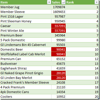
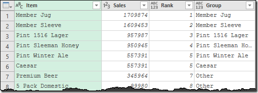
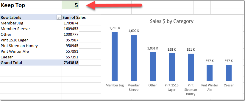
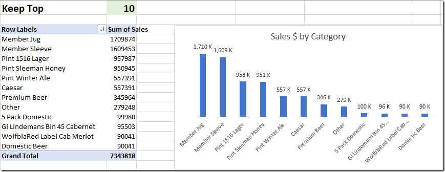
One thing I did incorporate here was that I added some extra ties a bit lower down, suggested by Kevin. This turned out to be super important, as it enabled me to validate that all the approaches were truly in sync (and fix them when they weren't). With the ability to change the "Top X" from a worksheet cell, we can now dynamically compare the results and see that they are the same. So the revised table now looks like this:
Apart from those little nuances, everything (with some small mods) fell neatly into the buckets. And all in all, I've got 5 different solutions to showcase that return the same result.
Laying the groundwork
Before jumping in to the techniques used to solve the Top X with Ties Challenge, I just want to lay out the groundwork I used to illustrate them all.
Groundwork - Dynamic portion
I wanted to be able to pull the Top X from a worksheet cell so that it was easy to update. To do this I:
- Created a named range called "rngKeep"
- Entered the value of 5
- Selected the cell and pulled it in to Power Query
- Renamed the query "TopX"
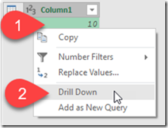
- Right clicked the whitespace beside my value --> Drill Down
- Loaded the query as a Connection (not to table)
And with that, we've now got the framework to dynamically update our Top X via a worksheet cell.
Groundwork - Staging Query
The next piece I needed was a simple base query to use to demo all the different techniques. To do this I:
- Selected a cell in the data table (which I had renamed to "Sales")
- Pulled the data into Power Query
- Change the Data Types to Text and Whole Number
- Sorted the rows in Descending Order based on the Sales column
- Renamed the query to SourceTable
- Loaded the query as a Connection
And that's it. We're now ready to explore the solutions that came in. ![]()
Top X with Ties Challenge - Solution 1 - Using Merges
We had a total of 3 submissions that used this method (including mine). This solution (as illustrated) requires two queries (although they could be merged into one if you wanted to):
Creating the TopXItems query
To do this you just need to:
- Reference the SourceTable
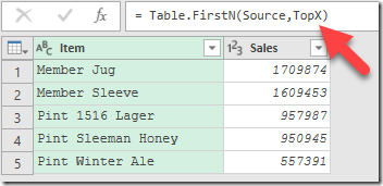
- Keep the top 5 rows, then replace the 5 in the formula bar with "TopX" that it can update dynamically
- Load it as a Connection only query (called TopXItems) for later use.
Creating the Grouping (via Merge) query
- Reference the SourceTable again
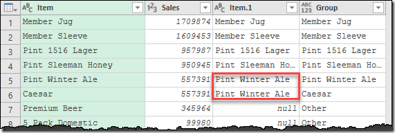
- Merge the Sales columns against the same column of the TopXItems query using a Left Outer join
- Expand the Item field from the new column
- Add a new Conditional Column that replicates the following logic:
- if [Item.1] = null then "Other" else [Item]
- Remove the [Item.1] column
- Select the Item and Sales columns (together) --> Remove Duplicates
- Load the data to the destination
Relatively easy and it works well. Just a quick note here about the duplicates part is that due to the join type you could end up duplicating values, so the removal is needed at the end.
Top X with Ties Challenge - Solution 2 - Using Grouping
Next up, we've got grouping as a method to work this out - a technique that was featured in 6 of the submitted examples in one form or another. Funny enough, I didn't solve my issue this way, although I think it has to be a front runner for solving this issue.
To solve the issue using this method:
- Add an Index column from 1
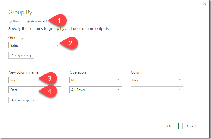
- Go to Transform --> Group --> Advanced
- Group by the Sales column
- Create a column called Rank to aggregate the Min from Index
- Create a column called Original to group All Rows
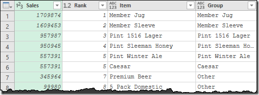
- Expand the [Item] field from the Data column
- Add a Custom Column to create the Group column using the following formula:
- if [Rank] <= TopX then [Item] else "Other"
- Remove the Rank column
- Reorder the columns (if desired)
- Load to the final destination
What I love about this is that it's super easy, 100% user interface driven and actually provides a lot of ability to play with the ranking.
I'll follow up on that last comment in a future post, including why I put the Index column where I did, and why it was part of the grouping (as I know some of you did this after grouping by Sales.) We'll devote an entire post to those nuances as they are important and I've got 3 more methods to cover.
Top X with Ties Challenge - Solution 3 - Using Chris Webb's Rankfx Function
This one was an interesting one, as it uses a technique that Chris Webb first wrote about back in 2014 in his Power Query book. (Note, this was not submitted by Chris!)
Here's how this query is built up:
- Reference the SourceTable query
- Click the fx in the Formula bar to get a new step and replace =Source with:
- = (SalesValue) => Table.RowCount(Table.SelectRows(Source, each [Sales]>SalesValue)) + 1
- Right click and rename the Custom1 to Rankfx
- Click the fx in the formula bar again, and =Rankfx with =Source
- Add a Custom Column using the following formula:
- =Rankfx([Sales])
- Remove the Rank Column
- Load to the final destination
I haven't checked with Chris, but I suspect that his technique precedes the existence of any UI to do grouping. (I know it precedes the UI for merging, as that wasn't in place when we wrote M is for Data Monkey.) Still, it works nicely to get the job done.
Top X with Ties Challenge - Solution 4 - Using List.Contains
While I wasn't the only one who drove to a List function to solve this issue, I was the only one that tried to do this by using a List.Contains function. My logic here was that list functions should be fast, and if I can check each line to see if it's included in the List, then I should be golden.
Creating the TopXList List
The first thing I needed was my list to examine. This was pretty easy to accomplish:
- Reference the SourceTable query
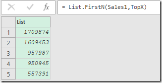
- Right click the Sales column header --> Drill Down
- List Tools --> Transform --> Keep Items --> Keep Top Items --> 5
- Replace 5 in the formula bar with TopX
- Rename to TopXList
- Load as a Connection
Note that because the original column is called Sales, the list seems to inherit a name of Sales1. I assume this is to disambiguate it in the code.
Grouping via List.Contains
Armed with my list, I could now figure out the grouping in a new query. To do this:
- Reference the SourceTable
- Add a Custom Column called Group using the following formula:
- if List.Contains(TopXList,[Sales]) then [Item] else "Other"
- Load the query to the final destination
I have to be honest, it surprised me how easy this was to do. Yes, I did need to do a quick bit of reading about the List.Contains function (since we don't have any Intellisense in Power Query yet), but overall, this was pretty slick to build. Using list functions, this should be very quick to execute and - if it needs more speed - I could always buffer the list as well. (With data this small it's irrelevant.)
The only thing I don't like about this one is that you do have to go and get jiggy with formulas. And if you're not comfortable reading MSDN documents (which tends to be code centric and poorly illustrated for Excel people), then you could end up getting turned off by this.
Top X with Ties Challenge - Solution 5 - Using List Drilldown
The final solution I'm showcasing is the only other list function that was submitted. This was submitted by Daniil and approaches the job a bit differently than I did. It's still amazingly simple at the end though. Broken down it has two parts:
- Identify the value representing the TopN value
- Run logic to change the description for items greater than the TopN value
Identifying the TopN item from the list
To get started, we can create the TopN as follows:
- Reference the SourceTable query
- Right click the Sales column --> Drill Down
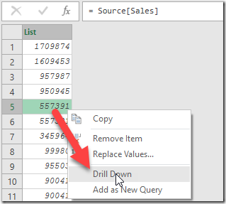
- Right click the row representing our max row --> Drill Down
- Replace the value (which will be one less than the row number pictured above) with "TopX-1"
- Rename the query to TopN
- Load as a Connection only
The key to remember here is that Power Query always counts from 0, which is why we need to subtract 1 from out TopX value when we are drilling in to the table to retrieve that item.
Adding a Group based on the TopN
With the TopN identified, we can now run some conditional logic against our original table to group our data appropriately:
- Reference the SourceTable
- Add a Custom Column called Group with the following formula
- =if [Sales] >= SaleN then [Item] else "Other"
- Load the table to the destination
And that's it. The only really tricky part in this is that you need to shift that TopX value by one when you're modifying the drill down. But apart from that, this is just as easy to build as any other of the solutions.
Final thoughts on the Top X with Ties Challenge
Again, the first thing I want to say here is how much I appreciate everyone sending in their solutions to the Top X with Ties Challenge. It's always awesome to see how others approach things, and you've got no idea what cool things you'd made me start thinking about. ![]()
The second thing, and it's kind of tied to the first, is how cool it is that we've got multiple approaches to do the same thing. I'm always fond of saying that there are at least 3 ways to do everything in Excel, and what's more is that I know what we've got here isn't an exhaustive list. How cool is that?
Feel free to download the illustrated solution that I've described above. Above the output table for each method is the first name for the people who submitted their solution (so you can see how I grouped you in on this). And if you want to test out the refresh, here's what you need to do:
- Change the value in cell F1
- Go to Data --> Refresh All
- Go to Data --> Refresh All (yes, a 2nd time… so it updates the PivotTable & PivotChart)
No matter which query results you're looking at, you'll see that they are identical.
Which will perform fastest? Honestly, I didn't test this with more than 300,000 rows of data. When I tested, there was no real difference in speed between the solutions.
Which method should we use? Great question, and I don't have an answer. The List function methods should be fast, but the grouping is VERY versatile and is going to be my recommended method going forward. I know this is cruel, but in a couple of weeks I'm going to put up a post as to why that is. Stay tuned for that one!
Let me know your thoughts and comments. Did anyone else pick up any new techniques here? Any challenges you'd like to see posted?




11 thoughts on “Results: Top X with Ties Challenge”
Now, the real question: What scenario would you need to do this for, rather than using TopN in your pivot table, which is also completely UI driven? That natively pulls in ties, as well.
The only thing I can think of is if you absolutely must present your results in a table (not a pivot table) and can't use Power BI.
Hi Matthew,
Actually, I did this originally because I wanted the data in Power BI. This wasn't strictly a TopN exercise... that would drop the "other" values. I wanted my top 5 (with ties), but wanted all other values grouped as "Other" so they still showed in my visual.
I know there is grouping in PowerBI, but last I checked you had to define those items by name. If the top 5 changes... the Power Query solution will update, a solution targeted at names won't.
Hello Ken,
Ah! That makes sense, still doable in DAX but much more complicated than any of the M solutions, true. I forgot you couldn't do a NOT TopN filter the way you can with the rest.
As usual, thanks again for the very intriguing M solutions!
You had me worried there for a minute. I was wondering if I overthought the issue! ?
Huh. The blog ate my LOL emoji and replaced it with a ? I thought it supported Emojis!
Hmm, I'm pretty sure the UI for merging was in place when I wrote that function - it's just that my code represents the way I'd naturally try to solve the problem. In fact when I read the original challenge I had forgotten about the solution in the book, but I do remember thinking that I'd probably use a function here...
Pingback: Creating Dynamic Parameters in Power Query - The Ken Puls (Excelguru) BlogThe Ken Puls (Excelguru) Blog
Pingback: Ranking Method Choices in Power Query - The Ken Puls (Excelguru) BlogThe Ken Puls (Excelguru) Blog
Pingback: Power Query Challenge #2 - The Ken Puls (Excelguru) BlogThe Ken Puls (Excelguru) Blog
Pingback: Ranking Method Choices in Power Query - Excelguru
Pingback: Challenge - Top x with Ties - Excelguru