Last week, in a blog comment, a reader asked how to filter their data to only show the most recent rolling 12 month period.  This post looks at how I made that work in Power Query.

Background

Assume we have a table set up as follows:

As you can see, we have sales categories down the left, months across the top, and values in the middle.  A classic setup when users are tracking information.  And now we need to pull the most recent 12 months only from that table.

You can download the completed sample file if you’d like to follow this along as well.

Filter the most recent rolling 12 months from a table in Power Query

Step 1: Grab the data

First thing we need to do is grab the data. To do this, I clicked in the table and:

• Power Query –> From Table –> Confirm the range (if required)
• Changed the query name to Rolling12

Helpfully, Power Query identified the data types in all the columns for me, so I’m pretty much ready to go.

Step 2: Show the most recent record first

To do this, we really need to get the data into an unpivoted list.  Easy enough to do:

• Select the “Sales” column
• Right click –> UnPivot Other Columns

Note: The “unpivot other columns” command was added to the right click menu in version 2.24.  While you can most likely still access this command, you are definitely running an older version, and for a multitude of important reasons, you should really update to the latest version of Power Query.

If you don’t want to (or can’t) do this for some reason, then go to Transform –> Unpivot –> Unpivot Other columns to accomplish the same thing.

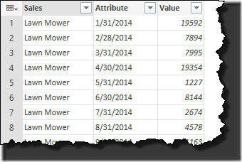
We now get a nice unpivoted list:

Next I cleaned up that Attribute column:

• Right click the Attribute column –> Rename –> Date
• Right click the Date column –> Changed Type –> Date

And finally I sorted the records to show the most recent ones at the top:

• Click the Filter icon on the Date column –> Sort Descending

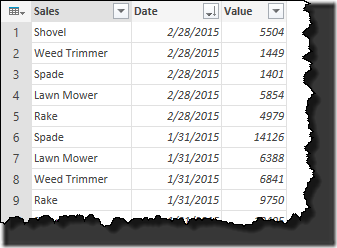
Leaving us with this:

Step 3: Create variables to hold the required data range

Next we need to work out the dates that we want to use for the top and bottom range of dates in the query.  This is a bit tricky, but uber powerful once you realize you can do it.

To start, click the fx icon in the formula bar:

NOTE: If you don’t see the formula bar, go to the View tab, and check the box next to Formula Bar

What this does is add a new step in the formula bar called “Custom1”.  And if you check the formula bar you’ll see that it just refers to the previous step:

The cool thing here is that we can modify this.  Why don’t we add some data to the end of that statement to pull the first value from the Date column of that table?  To do that, change the text in the formula bar to read as follows:

=#”Sorted Rows”[Date]{0}

Recognize here that:

• #”Sorted Rows” refers to the table in the previous step
• [Date] tells Power Query that you only want the Date column
• {0} tell Power Query that you want the first value from that column (remember that Power Query starts counting from 0)

The result is a single cell with the most recent date:

Let’s keep things clean in our Steps window… right click the Custom1 step and rename it to “MaxDate”.

What’s cool here is that we’ve essentially created a variable to work out and hold the most recent date.

So now that we have the top of the range, why don’t we create another step to modify it to the date for the lower end of the range?

• Click the fx step in the formula bar
• Modify the formula to read as follows

=Date.AddYears(MaxDate,-1)

And the result is a new Custom1 step that shows in the formula bar as follows:

Note:  The formulas you can use are documented at Microsoft’s site here: http://office.microsoft.com/en-us/excel-help/power-query-formula-categories-HA104122363.aspx

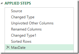
Pretty cool, don’t you think?  We’ve now got a step that holds the lower end of the results too.  Let’s do our cleanup again.

Right click the Custom1 step and rename it to “AfterDate”

Step 4: Implement the variables into a filter

Our last step is to implement the variables into the filter, cutting the data down to the most recent rolling 12 months of data.  Before we can do that, however, we really need to get back to the table we had in the “Sorted Rows” step.

The challenge is that we can’t select and work from that step, as it’s earlier in the process than the creation of our variables.  So how do we get back to that step AFTER we’ve created our variables?

• Click the fx button in the formula bar

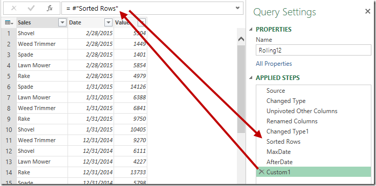
Once again, we get a new step in the formula bar:

The problem is that it’s referring to the previous step.  So what if we changed it to point to the #”Sorted Rows” step?

Now how cool is that?  Not only can we refer to the previous step of our query, we can change that to point to ANY previous step, or type in our own formulas against any previous step!

NOTE:  If your steps have spaces in the, don’t forget to wrap the step name in quotes and then preface it with the # symbol.  If your steps don’t have spaces, then you don’t need to do this.

Okay, so now let’s filter our data.  We’ll start by doing it manually:

• Click the filter icon on the Date column
• Select Date Filters –> Custom Filter
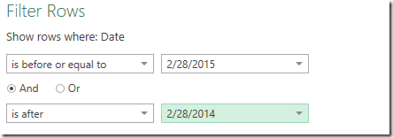
• Set up your filter as follows:

Notice that we have to pick the values from the list here.  (Wouldn’t it be cool if we could type in our variable names here?  That would be awesome!)  Regardless, we can set up the filter as we’d expect to use it.  This will filter our list, and leave us with the following formula in the formula bar:

NOTE:  You can expand the formula bar to show as I have by clicking the little down arrow icon.

Good stuff… now we need to do a little surgery.  Let’s replace the manual dates with our variables:

= Table.SelectRows(Custom1, each [Date] <= MaxDate and [Date] > AfterDate)

If you check the table now, you’ll see that it is filtered down to only contain records between Mar 1, 2014 and Feb 28, 2015.  And better yet, because the variables are created dynamically when the query is run, it will ALWAYS return the most recent rolling 12 months!

Step 5: Pivoting the data back into the original format.

Now we need to put the data back into the format the user wanted.  To do this, we need to pivot it back.

The trick to pivoting in Power Query is to select the column you want to use as the new column headers.  This time it is the Date column.  So…

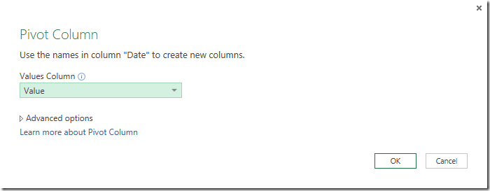
• Select the Date column –> Transform –> Pivot Column
• Change the “Values” column to the one that holds your values (in this case it’s actually called Value)

And the result:

Bingo!  The most recent rolling 12 months of data from our table.

At the point you can click File –> Close & Load, and load it to a table.

Proof Positive

Go and add a new column of data.  You can insert it into the existing table, put it on the end, it really doesn’t matter since Power Query will sort it anyway.  Once you’re done, right click the new table and refresh it, and you’ll find it works nicely.

One minor point of note… in the version I did we’ve actually reversed the column order (the most recent date has moved to the left from the right.)  If we wanted to change that it’s fairly easy too.  Just before we pivot the data back into the pivoted form, just sort it in descending order.