I was fooling around with the latest build of Power Query (for Excel 2010/2013), and I’ve got to say that I’m actually really impressed with this piece. I think the user experience still needs a bit of work, but once you know how, this is really simple.
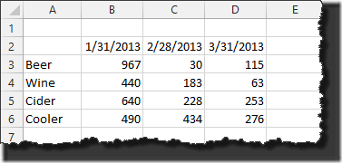
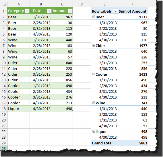
Whenever I teach courses on PivotTables people want to eat them up, but often they’ve already got their data in a format that resembles the PivotTable output, rather than a format that is consumable by the Pivot engine. Take the following set of data.
A classic setup for how people think and want to see the data. But now what if the user wanted to see the records by month under the category breakdowns? An easy task for a Pivot, but it would require a bit of manipulation without it. So how do we get it back to a Pivot compliant format?
With Power Query it’s actually super simple:
- Step 1: Select the data and turn it into a table
- Step 2: Select Power Query –> From Table to suck it in to Power Query
- Step 3: Un-pivot it
Okay, so this one takes a bit of know how right now. If you just click Unpivot, you get something really weird:
What actually needs to happen, which isn’t totally intuitive, is we need to click the header for the January column, hold down CTRL and click the February and March column headers:
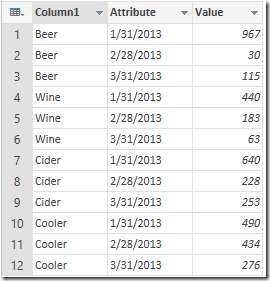
Once we’ve done that we click Unpivot and TA-DA!
So by virtue of being able to choose one or more columns, it’s actually quite flexible as you can choose HOW to un-pivot, which is uber-awesome. It’s a shame the UI doesn’t help you realize that today, but hopefully that gets fixed in future.
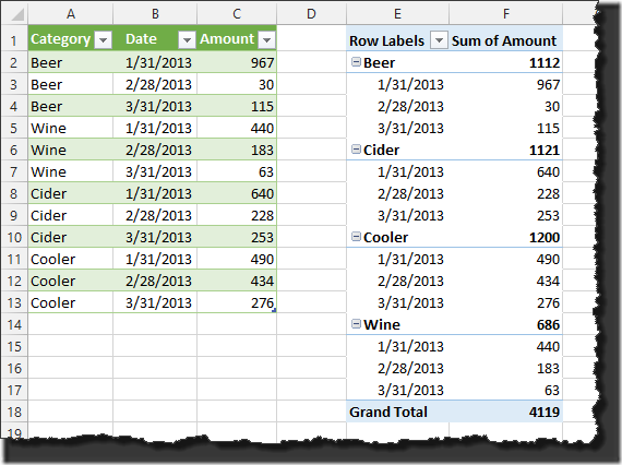
At any rate, you can right click the headers to rename the columns, then click “Apply and Close” and we end up with the un-pivoted source in our worksheet. And now we can create a new PivotTable off that source:
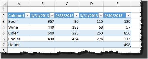
Even better, if we add some new data to our original report:
We can then refresh the query on the worksheet and the records are pulled in. With a refresh on the Pivot as well (yeah, unfortunately you can’t just refresh the pivot to drive the query to update) it’s all pulled in:
Pretty damn cool!




15 thoughts on “Un-Pivoting Data in Power Query”
Pingback: Excel Roundup 20131118 | Contextures Blog
Hi Ken,
Using a pivot table you can do this too.
1. Add the pivot table wizard to your QAT or prees alt+d,p
2. Select Mutliple consolidation ranges
3. Click next and leave the default selected and click next again.
4. Select your table and click Add
5. Click Finish
6. Double-click the Grand total cell bottom-right of the pivot table.
That's true, Jan Karel. But once you started needing the super secret Excel MVP handshake or decoder ring to find the feature it became pretty inaccessible to most people. (Not that it was really discoverable being hidden where it was in that setup either.) This brings the feature up front and centre, which is much better, IMO. 🙂
Pingback: Daily Dose of Excel » Blog Archive » UnPivot via SQL
Good stuff, Ken. I haven't played around with this much, because I don't have it at work. So hard to justify the time when there's plenty of stuff in good-ol VBA that I can learn on the Boss' dime 🙂
Hey, just did a related post over at DDOE on how to do an UnPivot using SQL. Check it out.
@Ken: at least now the handshake isn't secret anymore, as it is going to live on forever as a comment to this post! 🙂
Pingback: Pivoting Data In Power Query | Chris Webb's BI Blog
Great article, but I need to take the unpivot one step further, is it possible to unpivot sub catagories, So for your example, if 1/31, 2/28, and 3/31 had sub categories of x,y, and z. How would you unpivot?
Pingback: Unpivot Nested Headings With Power Query | Bob's BI Ramblings
Oh man... sorry to be so late on this reply. Yes, we can do that. I posted a blog post today on how to make this happen: https://excelguru.ca/2014/09/24/un-pivoting-with-subcategories-in-power-query/
Pingback: Transform already-pivoted tables to PivotTable (The Definitive Guide to Unpivot with Power Query in Excel) - Get & Transform Data in Excel 2016 - Site Home - TechNet Blogs
Pingback: Transform already-pivoted tables to PivotTable (The Definitive Guide to Unpivot with Power Query in Excel) | Data Chant
Nice post, Ken.
One query, if we have multiple paired columns and want to make single pair then how to do it.
Say My row data has say around 10 pairs (showing here only 3),
GroupA GroupB GroupC
Name Score Name Score Name Score
A1 10 B1 11 C1 50
A2 20 B2 15 C2 16
A3 30 B3 19 C3 39
Now if I want to convert it with three columns like
Group Name Score
GroupA A1 10
GroupA A2 20
GroupA A3 30
GroupB B1 11
GroupB B2 15
and so on....................
Hi Vijay,
Check out this post: https://excelguru.ca/2014/09/24/un-pivoting-with-subcategories-in-power-query/
Cheers!
Pingback: Un-pivoting With Subcategories in Power Query