Use Excel Tables to Filter a Power Query

A question came up in the Excelguru forums today about how to use Excel tables to filter a Power Query.  While Power Query can't read a filter from an Excel table natively, there is a cool little trick that you can do to flow that information through, though.

Data Background

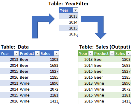
The data footprint I'm working with looks like this:

The Data query is a fairly simple staging query, pulling the data from the Excel table on the left, setting data types, and loading as Connection Only.

The YearFilter query is a little more complicated, as it pulls the data, removes duplicates, and then drills down into the Year column (right click the header -> Drill Down), resulting in a unique list of the Years:

And finally the Sales Query, which - shown in an indented and 'colourfied' format thanks to Monkey Tools' QuerySleuth - looks like this:

The important things to notice about this query are:

• It references the Data query (no new data is added here)
• The Filtered Rows step filters to include any item that is in the list generated by the YearFilter list
• The Filtered Rows step had to be adjusted manually to add the List.Contains function
• The [Year] column refers to the [Year] column of the Sales query (which flows through from the original data)

So What's the Issue?

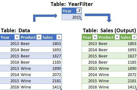
We want to use the filter on the YearFilter table in Excel to filter our Power Query.  Unfortunately, that doesn't happen... despite a refresh, all the years are still in the worksheet after setting that filter:

The challenge, when you are attempting to use Excel tables to filter a Power Query, is that Excel can't read the filter.  In fact, Power Query can't access any of the table's metadata about filters or the visible state of the rows.  It therefore brings in all rows from the table whether they are hidden or not.

Using Excel Tables to Filter a Power Query

The secret here is that we need a way to tell Power Query which rows are visible versus which are hidden.  Something we can do by leveraging the AGGREGATE function, since it has the ability to count only visible rows.

The formula I used was =AGGREGATE(3,5,[@Year]) where:

• 3 indicates the COUNTA() function
• 5 sets it to ignore Hidden rows
• [@Year] points to the current row of the Year column

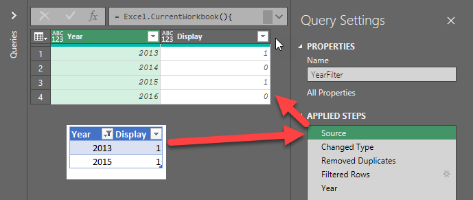
The weird part, if you've never done this before, is that all the visible rows in Excel will always show a 1. But look what happens when you filter to only a couple of years, then edit the YearFilter Query and select the Source step: Boom!  We can see which rows are visible (indicated with a 1) and which are hidden (indicated with a 0).  This now becomes a pretty easy fix:

• Filter the Display column to 1

And you're done.  The rest of the query will still work, as it drills in to the list of years, so we don't even need to remove this new column.

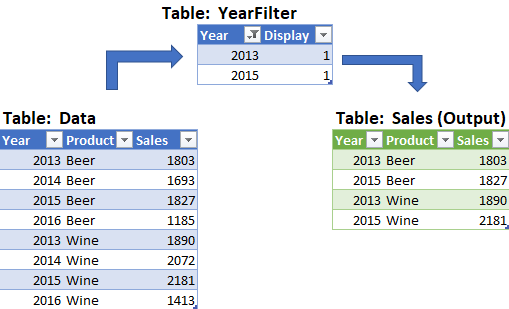
And just like that, we can now use Excel tables to filter a Power Query: